Qiskit 소개#
Qiskit을 사용하는 경우 사용자 워크플로우는 다음의 네 가지 상위 레벨 단계로 구성된다.
Build: 사용자가 고려하고 있는 문제를 나타내는 양자 회로(들) 을 설계한다.
Compile: 특정 양자 서비스를 위한 회로를 컴파일한다 (예: 양자 시스템 또는 고전 시뮬레이터).
Run: 지정된 양자 서비스에서 컴파일된 회로를 실행한다. 이러한 서비스는 클라우드 기반 또는 로컬일 수 있다.
Analyze: 요약적인 통계를 계산하고 실험 결과를 시각화한다.
자세한 설명과 함께 각각의 단계와 전체 작업 흐름을 보여주는 예제를 살펴보자.
from qiskit import QuantumCircuit, transpile
from qiskit_aer import AerSimulator
from qiskit.visualization import plot_histogram

# Use Aer's AerSimulator
simulator = AerSimulator()

# Create a Quantum Circuit acting on the q register
circuit = QuantumCircuit(2, 2)

# Add a H gate on qubit 0
circuit.h(0)

# Add a CX (CNOT) gate on control qubit 0 and target qubit 1
circuit.cx(0, 1)

# Map the quantum measurement to the classical bits
circuit.measure([0, 1], [0, 1])

# Compile the circuit for the support instruction set (basis_gates)
# and topology (coupling_map) of the backend
compiled_circuit = transpile(circuit, simulator)

# Execute the circuit on the aer simulator
job = simulator.run(compiled_circuit, shots=1000)

# Grab results from the job
result = job.result()

# Returns counts
counts = result.get_counts(compiled_circuit)
print("\nTotal count for 00 and 11 are:", counts)

# Draw the circuit
circuit.draw("mpl")

# Plot a histogram
plot_histogram(counts)
순차적 작업 흐름#
위의 프로그램은 다음의 여섯 단계로 나누어 질 수 있다.
패키지 가져오기
변수 초기화
게이트 추가
회로 시각화
실험 시뮬레이션
결과 시각화
1단계: 패키지 가져오기#
프로그램에 필요한 기본적인 요소들은 다음과 같이 가져올 수 있다:
from qiskit import QuantumCircuit
from qiskit_aer import AerSimulator
from qiskit.visualization import plot_histogram
보다 자세히 설명하면, 가져올 패키지들은
QuantumCircuit: 양자 시스템의 설명서로 생각할 수 있다. 여기에는 모든 양자 연산이 포함된다.AerSimulator: Aer 의 고성능 회로 시뮬레이터이다.plot_histogram: 히스토그램을 생성한다.
2단계: 변수 초기화#
다음 코드의 줄을 보자
circuit = QuantumCircuit(2, 2)
여기 2개의 큐비트를 0 상태로 초기화하고, 2개의 고전적인 비트를 0으로 초기화 하는 경우를 생각해 보자. circuit 은 양자 회로를 말한다.
구문:
QuantumCircuit(int, int)
3단계: 게이트 추가하기#
게이트들을 (연산들을) 추가하여 회로의 레지스터들을 조작할 수 있다.
다음 세 줄의 코드를 참고하자:
circuit.h(0)
circuit.cx(0, 1)
circuit.measure([0, 1], [0, 1])
게이트들이 회로에 하나씩 추가되어 Bell 상태를 만들고 있다.
위의 코드는 다음의 게이트들을 적용한다:
QuantumCircuit.h(0): 하다마드 게이트 \(H\), 큐비트 0을 중첩 상태 로 만든다.QuantumCircuit.cx(0, 1): 제어 반전 게이트 (\(CNOT\)), 조절 큐비트 0과 표적 큐비트 1을 얽힘 상태 로 만든다.QuantumCircuit.measure([0,1], [0,1]): 모든 양자와 클래식 레지스터들을측정한다면, i 번째 큐비트의 측정 결과는 i 번째 클래식 비트에 저장될 것이다.
4단계: 회로 시각화하기#
직접 디자인한 회로를 많은 교과서 및 연구 자료에서 사용되는 다양한 형태들로 보기 위해서 qiskit.circuit.QuantumCircuit.draw() 를 사용할 수 있다.
circuit.draw("mpl")
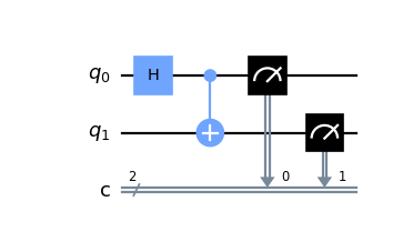
이 회로에서는 큐비트 0은 위쪽에, 큐비트 1은 아래쪽에 가도록 정렬되어 있다. 회로는 왼쪽에서 오른쪽으로 읽는데, 이것은 가장 왼쪽의 게이트들이 회로에서 먼저 적용된다는 것을 의미한다.
QuantumCircuit.draw() 나 qiskit.visualization.circuit_drawer() 에 사용되는 기본 백엔드는 텍스트 백엔드이다. 하지만 당신의 로컬 환경에 따라 필요에 맞는 좀 더 적절한 백엔드를 사용하고 싶을 수 있다. 이는 사용자 환경 파일을 통해 변경이 가능하다. 기본적으로 사용자 환경 파일은 ~/.qiskit/settings.conf 디렉토리에 저장되어야 하고 .ini 확장자를 가져야 한다.
예를 들어, Matplotlib 그리기 설정을 위한 settings.conf 파일은 다음과 같다:
[default]
circuit_drawer = mpl
이 설정의 값으로 아무 종류의 유효한 회로 그리기 백엔드를 사용할 수 있는데, text, mpl, latex, 그리고 latex_source 등이 이에 해당된다.
5단계: 실험 시뮬레이션 하기#
Qiskit Aer is a high performance simulator framework for quantum circuits. It provides several backends to achieve different simulation goals.
If you have issues installing Aer, you can alternatively use the Basic Aer provider by replacing Aer with BasicAer. Basic Aer is included in Qiskit.
from qiskit import QuantumCircuit, transpile
from qiskit.providers.basicaer import QasmSimulatorPy
...
이 회로를 시뮬레이션하기 위해서 AerSimulator 를 사용할 예정이다. 이 회로의 각 실행 결과로 00 혹은 11 비트 문자열이 나올 것이다.
simulator = AerSimulator()
compiled_circuit = transpile(circuit, simulator)
job = simulator.run(compiled_circuit, shots=1000)
result = job.result()
counts = result.get_counts(circuit)
print("\nTotal count for 00 and 11 are:",counts)
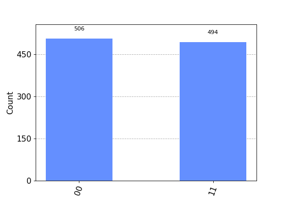
예상한 대로 출력 비트 문자열 00은 대략 50 퍼센트의 확률로 확인할 수 있었다. 회로가 몇 번 실행될 것인가는 execute 함수의 shots 인수로 설정할 수 있다. 이 시뮬레이션의 샷 수는 1000으로 설정되었다 (기본값은 1024이다).
result 객체를 얻은 후에는 시뮬레이션 결과값 통계를 get_counts(circuit) 함수를 통해 얻을 수 있다. 이를 통해 지금까지 실행했던 실험들의 합계된 결과를 확인할 수 있다.
6단계: 결과 시각화하기#
Qiskit 은 결과를 보여주기 위해 많은 시각화 방법들을 제공한다.
이중에는 plot_histogram 함수도 포함되어 있다.
plot_histogram(counts)
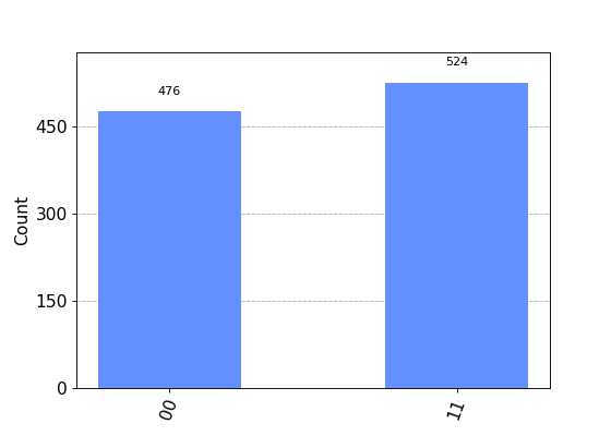
관측된 확률 \(Pr(00)\) 와 \(Pr(11)\) 는 각각의 값이 나온 실험의 수를 총 샷 수로 나누어 계산되었다.
참고
run() 메서드의 shots 전달 인자를 바꿔서 입력해 보고 각각의 경우에 따라 예상되는 확률이 어떻게 변하는 지를 확인해 보라.
다음 단계#
이제 기본기를 익혔으므로, 다음 학습 자료들을 참고할 수 있다: