Qiskit 入門#
Qiskitを使用する際、ユーザーのワークフローは主に以下4つの大まかなステップから構成されます。
ビルド:検討している問題を表す量子回路を設計します。
コンパイル:特定の量子サービス(量子システムや古典シミュレーターなど)のために回路をコンパイルします。
実行:コンパイルされた回路を、指定された量子サービス上で実行します。これらのサービスは、クラウドベースでもローカルでも構いません。
分析:統計情報を計算し、実験結果を可視化します。
以下にワークフロー全体の例を示します。各ステップの詳細は後のセクションで説明します。
from qiskit import QuantumCircuit, transpile
from qiskit_aer import AerSimulator
from qiskit.visualization import plot_histogram

# Use Aer's AerSimulator
simulator = AerSimulator()

# Create a Quantum Circuit acting on the q register
circuit = QuantumCircuit(2, 2)

# Add a H gate on qubit 0
circuit.h(0)

# Add a CX (CNOT) gate on control qubit 0 and target qubit 1
circuit.cx(0, 1)

# Map the quantum measurement to the classical bits
circuit.measure([0, 1], [0, 1])

# Compile the circuit for the support instruction set (basis_gates)
# and topology (coupling_map) of the backend
compiled_circuit = transpile(circuit, simulator)

# Execute the circuit on the aer simulator
job = simulator.run(compiled_circuit, shots=1000)

# Grab results from the job
result = job.result()

# Returns counts
counts = result.get_counts(compiled_circuit)
print("\nTotal count for 00 and 11 are:", counts)

# Draw the circuit
circuit.draw("mpl")
# Plot a histogram
plot_histogram(counts)
ワークフローのステップバイステップ#
上のプログラムは6つの手順に分解できます。
パッケージのインポート
変数の初期化
ゲートの追加
回路の可視化
実験のシミュレーション
結果の可視化
ステップ 1 : パッケージのインポート#
プログラムに必要な基本的要素は以下のようにインポートされます。
from qiskit import QuantumCircuit
from qiskit_aer import AerSimulator
from qiskit.visualization import plot_histogram
インポートされるものの詳細は以下の通りです。
QuantumCircuit: 量子システムの命令と考えることができます。すべての量子演算を行うことができます。AerSimulator: Aerによる高性能な回路シミュレーターです。plot_histogram: ヒストグラムを作成します。
ステップ2:変数の初期化#
次のコードを考えてみます。
circuit = QuantumCircuit(2, 2)
ここでは、二つの量子ビットをゼロの状態に、二つの古典ビットをゼロに初期化し、量子回路 circuit に代入しています。
構文:
QuantumCircuit(int, int)
ステップ3:ゲートの追加#
ゲート(演算)を追加することで、回路のレジスタを操作することができます。
次の3行のコードを考えてみましょう。
circuit.h(0)
circuit.cx(0, 1)
circuit.measure([0, 1], [0, 1])
ゲートは1つずつ回路に追加され、ベル状態を形成します。
上記のコードは、以下のゲートを適用しています。
QuantumCircuit.h(0): 量子ビット0にアダマールゲート \(H\) を設定し、 重ね合わせ状態 にします。QuantumCircuit.cx(0, 1): 制御量子ビット0とターゲット量子ビット1に対する制御NOT演算( \(CNOT\) )で、量子ビットを エンタングル状態 にします。QuantumCircuit.measure([0,1], [0,1]): 量子レジスタと古典レジスタの全体をmeasureに渡すと、i番目の量子ビットの測定結果がi番目の古典ビットに格納されます.
ステップ4:回路の可視化#
qiskit.circuit.QuantumCircuit.draw() を使用して、多くの教科書や研究記事で使用されているさまざまな形式で設計した回路を表示できます。
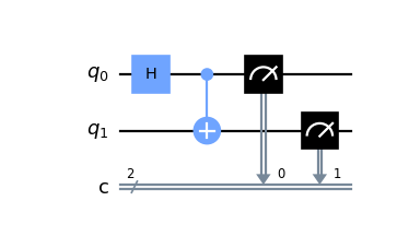
circuit.draw("mpl")

この回路では、量子ビットは量子ビット0が上、量子ビット1が下に記述されています。回路は左から右に読み、左に表示されているゲートから順に適用されます。
QuantumCircuit.draw() 又は qiskit.visualization.circuit_drawer() のデフォルトのバックエンドは text backendです。あなたのローカル環境によっては、より適切なデフォルトの設定を行う必要があるかもしれません。その場合はuser configファイルの設定を行うことで対応できます。user configファイルは通常 ~/.qiskit/settings.conf 下の .ini ファイルになります。
例えば, Matplotlib drawer を設定するための settings.conf ファイルは:
[default]
circuit_drawer = mpl
このconfigには、有効な circuit drawer バックエンドであればどれでも指定することができます。これらには text, mpl, latex, そして latex_source が含まれます。
ステップ 5 : 実験のシミュレーション#
Qiskit Aer is a high performance simulator framework for quantum circuits. It provides several backends to achieve different simulation goals.
If you have issues installing Aer, you can alternatively use the Basic Aer provider by replacing Aer with BasicAer. Basic Aer is included in Qiskit.
from qiskit import QuantumCircuit, transpile
from qiskit.providers.basicaer import QasmSimulatorPy
...
回路をシミュレートするためには、 AerSimulator を使用します。回路の実行毎にビット文字列00もしくは11を生成します。
simulator = AerSimulator()
compiled_circuit = transpile(circuit, simulator)
job = simulator.run(compiled_circuit, shots=1000)
result = job.result()
counts = result.get_counts(circuit)
print("\nTotal count for 00 and 11 are:",counts)
期待通りにビット文字列の出力が00になるのはだいたい50%です。回路の実行回数は execute メソッドの shots 引数で指定できます。このシミュレーションの実行回数は1000(デフォルトは1024) に設定されています。
result オブジェクトを取得できたら、get_counts(circuit) メソッドを使用して回数を取得することができます。実行した実験の総計を得ることができます。
ステップ6:結果の可視化#
Qiskitは 多くのビジュアライゼーション を提供します。
その中には結果を表示するための plot_histogram という関数も含まれます。
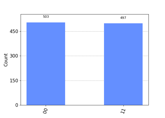
plot_histogram(counts)
観測された確率 \(Pr(00)\) と \(Pr(11)\) は、対応する事象が観測された回数を全実行回数で割った数値です。
注釈
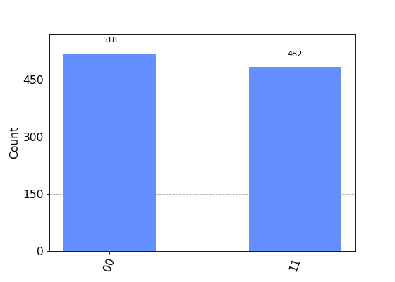
run() メソッドの shots 引数を変更して、推定される確率がどのように変化するか見てみましょう。
次のステップ#
基礎の学習が終わりました。次は、以下の学習リソースがあります。