Compute circuit output probabilities with Sampler primitive#
This guide shows how to get the probability distribution of a quantum circuit with the Sampler primitive.
Nota
While this guide uses Qiskit’s reference implementation, the Sampler primitive can be run with any provider using BackendSampler.
from qiskit.primitives import BackendSampler
from <some_qiskit_provider> import QiskitProvider

provider = QiskitProvider()
backend = provider.get_backend('backend_name')
sampler = BackendSampler(backend)
There are some providers that implement primitives natively (see this page for more details).
Initialize quantum circuits#
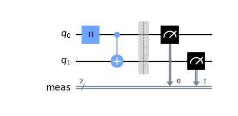
The first step is to create the QuantumCircuits from which you want to obtain the probability distribution.
from qiskit import QuantumCircuit

qc = QuantumCircuit(2)
qc.h(0)
qc.cx(0,1)
qc.measure_all()
qc.draw("mpl")
Nota
The QuantumCircuit you pass to Sampler has to include measurements.
Initialize the Sampler#
Then, you need to create a Sampler instance.
from qiskit.primitives import Sampler

sampler = Sampler()
Run and get results#
Now that you have defined your sampler, you can run it by calling the run() method,
which returns an instance of PrimitiveJob (subclass of JobV1). You can get the results from the job (as a SamplerResult object)
with the result() method.
job = sampler.run(qc)
result = job.result()
print(result)
SamplerResult(quasi_dists=[{0: 0.4999999999999999, 3: 0.4999999999999999}], metadata=[{}])
While this example only uses one QuantumCircuit, if you want to sample multiple circuits you can
pass a list of QuantumCircuit instances to the run() method.
Get the probability distribution#
From these results you can extract the quasi-probability distributions with the attribute quasi_dists.
Even though there is only one circuit in this example, quasi_dists returns a list of QuasiDistributions.
result.quasi_dists[i] is the quasi-probability distribution of the i-th circuit.
Nota
A quasi-probability distribution differs from a probability distribution in that negative values are also allowed. However the quasi-probabilities must sum up to 1 like probabilities. Negative quasi-probabilities may appear when using error mitigation techniques.
quasi_dist = result.quasi_dists[0]
print(quasi_dist)
{0: 0.4999999999999999, 3: 0.4999999999999999}
Probability distribution with binary outputs#
If you prefer to see the output keys as binary strings instead of decimal numbers, you can use the
binary_probabilities() method.
print(quasi_dist.binary_probabilities())
{'00': 0.4999999999999999, '11': 0.4999999999999999}
Parameterized circuit with Sampler#
The Sampler primitive can be run with unbound parameterized circuits like the one below.
You can also manually bind values to the parameters of the circuit and follow the steps
of the previous example.
from qiskit.circuit import Parameter

theta = Parameter('θ')
param_qc = QuantumCircuit(2)
param_qc.ry(theta, 0)
param_qc.cx(0,1)
param_qc.measure_all()
print(param_qc.draw())
        ┌───────┐      ░ ┌─┐
   q_0: ┤ Ry(θ) ├──■───░─┤M├───
        └───────┘┌─┴─┐ ░ └╥┘┌─┐
   q_1: ─────────┤ X ├─░──╫─┤M├
                 └───┘ ░  ║ └╥┘
meas: 2/══════════════════╩══╩═
                          0  1
The main difference from the previous case is that now you need to specify the sets of parameter values
for which you want to evaluate the expectation value as a list of lists of floats.
The i-th element of the outer list is the set of parameter values
that corresponds to the i-th circuit.
import numpy as np

parameter_values = [[0], [np.pi/6], [np.pi/2]]

job = sampler.run([param_qc]*3, parameter_values=parameter_values)
dists = job.result().quasi_dists

for i in range(3):
    print(f"Parameter: {parameter_values[i][0]:.5f}\t Probabilities: {dists[i]}")
Parameter: 0.00000   Probabilities: {0: 1.0}
Parameter: 0.52360   Probabilities: {0: 0.9330127018922194, 3: 0.0669872981077807}
Parameter: 1.57080   Probabilities: {0: 0.5000000000000001, 3: 0.4999999999999999}
Change run options#
Your workflow might require tuning primitive run options, such as the amount of shots.
By default, the reference Sampler class performs an exact statevector
calculation based on the Statevector class. However, this can be
modified to include shot noise if the number of shots is set.
For reproducibility purposes, a seed will also be set in the following examples.
There are two main ways of setting options in the Sampler:
Set keyword arguments for run()#
If you only want to change the settings for a specific run, it can be more convenient to
set the options inside the run() method. You can do this by
passing them as keyword arguments.
job = sampler.run(qc, shots=2048, seed=123)
result = job.result()
print(result)
SamplerResult(quasi_dists=[{0: 0.5205078125, 3: 0.4794921875}], metadata=[{'shots': 2048}])
Modify Sampler options#
If you want to keep some configuration values for several runs, it can be better to
change the Sampler options. That way you can use the same
Sampler object as many times as you wish without having to
rewrite the configuration values every time you use run().
Modify existing Sampler#
If you prefer to change the options of an already-defined Sampler, you can use
set_options() and introduce the new options as keyword arguments.
sampler.set_options(shots=2048, seed=123)

job = sampler.run(qc)
result = job.result()
print(result)
SamplerResult(quasi_dists=[{0: 0.5205078125, 3: 0.4794921875}], metadata=[{'shots': 2048}])
Define a new Sampler with the options#
If you prefer to define a new Sampler with new options, you need to
define a dict like this one:
options = {"shots": 2048, "seed": 123}
And then you can introduce it into your new Sampler with the
options argument.
sampler = Sampler(options=options)

job = sampler.run(qc)
result = job.result()
print(result)
SamplerResult(quasi_dists=[{0: 0.5205078125, 3: 0.4794921875}], metadata=[{'shots': 2048}])