Simulators

Introduction

This notebook shows how to import Qiskit Aer simulator backends and use them to execute ideal (noise free) Qiskit Terra circuits.

import numpy as np

# Import Qiskit
from qiskit import QuantumCircuit, QuantumRegister, ClassicalRegister
from qiskit import Aer, execute
from qiskit.tools.visualization import plot_histogram, plot_state_city

Qiskit Aer simulator backends

Qiskit Aer currently includes three high performance simulator backends: * QasmSimulator: Allows ideal and noisy multi-shot execution of qiskit circuits and returns counts or memory * StatevectorSimulator: Allows ideal single-shot execution of qiskit circuits and returns the final statevector of the simulator after application * UnitarySimulator: Allows ideal single-shot execution of qiskit circuits and returns the final unitary matrix of the circuit itself. Note that the circuit cannot contain measure or reset operations for this backend

These backends are found in the Aer provider with the names qasm_simulator, statevector_simulator and unitary_simulator, respectively.

# List Aer backends
Aer.backends()

[<QasmSimulator('qasm_simulator') from AerProvider()>,
 <StatevectorSimulator('statevector_simulator') from AerProvider()>,
 <UnitarySimulator('unitary_simulator') from AerProvider()>,
 <PulseSimulator('pulse_simulator') from AerProvider()>]

The simulator backends can also be directly imported from qiskit.providers.aer

from qiskit.providers.aer import QasmSimulator, StatevectorSimulator, UnitarySimulator

QasmSimulator

The QasmSimulator backend is designed to mimic an actual device. It executes a Qiskit QuantumCircuit and returns a count dictionary containing the final values of any classical registers in the circuit. The circuit may contain gates, measurements, resets, conditionals, and other advanced simulator options that will be discussed in another notebook.

Simulating a quantum circuit

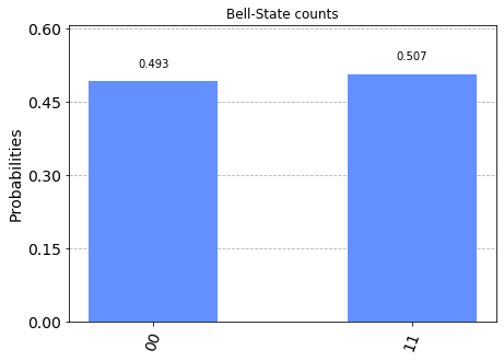
The basic operation executes a quantum circuit and returns a counts dictionary of measurement outcomes. Here we execute a simple circuit that prepares a 2-qubit Bell-state \(|\psi\rangle = \frac{1}{2}(|0,0\rangle + |1,1 \rangle)\) and measures both qubits.

# Construct quantum circuit
circ = QuantumCircuit(2, 2)
circ.h(0)
circ.cx(0, 1)
circ.measure([0,1], [0,1])

# Select the QasmSimulator from the Aer provider
simulator = Aer.get_backend('qasm_simulator')

# Execute and get counts
result = execute(circ, simulator).result()
counts = result.get_counts(circ)
plot_histogram(counts, title='Bell-State counts')

Returning measurement outcomes for each shot

The QasmSimulator also supports returning a list of measurement outcomes for each individual shot. This is enabled by setting the keyword argument memory=True in the assemble or execute function.

# Construct quantum circuit
circ = QuantumCircuit(2, 2)
circ.h(0)
circ.cx(0, 1)
circ.measure([0,1], [0,1])

# Select the QasmSimulator from the Aer provider
simulator = Aer.get_backend('qasm_simulator')

# Execute and get memory
result = execute(circ, simulator, shots=10, memory=True).result()
memory = result.get_memory(circ)
print(memory)

['00', '00', '00', '11', '11', '00', '00', '11', '11', '00']

Starting simulation with a custom initial state

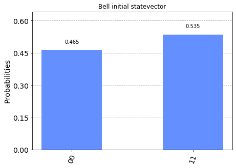
The QasmSimulator allows setting a custom initial statevector for the simulation. This means that all experiments in a Qobj will be executed starting in a state \(|\psi\rangle\) rather than the all zero state \(|0,0,..0\rangle\). The custom state may be set in the circuit using the initialize method.

Note: * The initial statevector must be a valid quantum state \(|\langle\psi|\psi\rangle|=1\). If not, an exception will be raised. * The simulator supports this option directly for efficiency, but it can also be unrolled to standard gates for execution on actual devices.

We now demonstrate this functionality by setting the simulator to be initialized in the final Bell-state of the previous example:

# Construct a quantum circuit that initialises qubits to a custom state
circ = QuantumCircuit(2, 2)
circ.initialize([1, 0, 0, 1] / np.sqrt(2), [0, 1])
circ.measure([0,1], [0,1])

# Select the QasmSimulator from the Aer provider
simulator = Aer.get_backend('qasm_simulator')

# Execute and get counts
result = execute(circ, simulator).result()
counts = result.get_counts(circ)
plot_histogram(counts, title="Bell initial statevector")

StatevectorSimulator

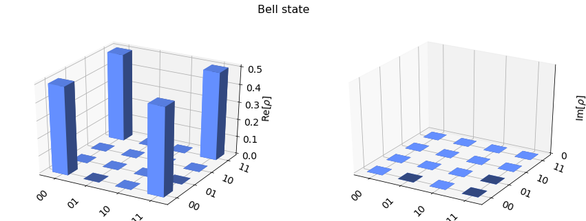
The StatevectorSimulator executes a single shot of a Qiskit QuantumCircuit and returns the final quantum statevector of the simulation. The circuit may contain gates, and also measurements, resets, and conditional operations.

Simulating a quantum circuit

The basic operation executes a quantum circuit and returns a counts dictionary of measurement outcomes. Here we execute a simple circuit that prepares a 2-qubit Bell-state \(|\psi\rangle = \frac{1}{2}(|0,0\rangle + |1,1 \rangle)\) and measures both qubits.

# Construct quantum circuit without measure
circ = QuantumCircuit(2)
circ.h(0)
circ.cx(0, 1)

# Select the StatevectorSimulator from the Aer provider
simulator = Aer.get_backend('statevector_simulator')

# Execute and get counts
result = execute(circ, simulator).result()
statevector = result.get_statevector(circ)
plot_state_city(statevector, title='Bell state')

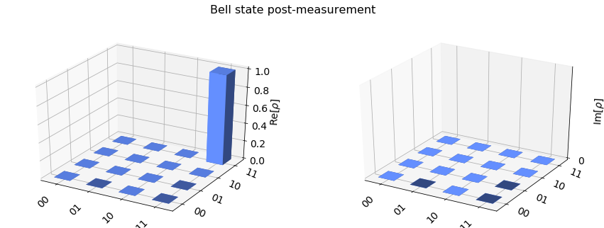
Simulating a quantum circuit with measurement

Note that if a circuit contains measure or reset the final statevector will be a conditional statevector after simulating wave-function collapse to the outcome of a measure or reset. For the Bell-state circuit this means the final statevector will be either \(|0,0\rangle\) or \(|1, 1\rangle\).

# Construct quantum circuit with measure
circ = QuantumCircuit(2, 2)
circ.h(0)
circ.cx(0, 1)
circ.measure([0,1], [0,1])

# Select the StatevectorSimulator from the Aer provider
simulator = Aer.get_backend('statevector_simulator')

# Execute and get counts
result = execute(circ, simulator).result()
statevector = result.get_statevector(circ)
plot_state_city(statevector, title='Bell state post-measurement')

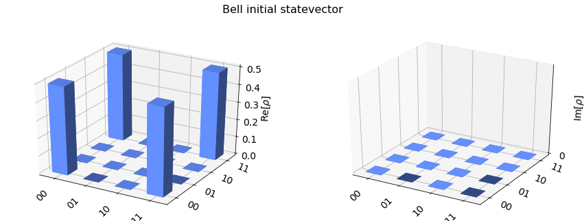
Starting simulation with a custom initial state

Like the QasmSimulator, the StatevectorSimulator also allows setting a custom initial statevector for the simulation. Here we run the previous initial statevector example on the StatevectorSimulator and initialize it to the Bell state.

# Construct a quantum circuit that initialises qubits to a custom state
circ = QuantumCircuit(2)
circ.initialize([1, 0, 0, 1] / np.sqrt(2), [0, 1])

# Select the StatevectorSimulator from the Aer provider
simulator = Aer.get_backend('statevector_simulator')

# Execute and get counts
result = execute(circ, simulator).result()
statevector = result.get_statevector(circ)
plot_state_city(statevector, title="Bell initial statevector")

Unitary Simulator

The UnitarySimulator constructs the unitary matrix for a Qiskit QuantumCircuit by applying each gate matrix to an identity matrix. The circuit may only contain gates, if it contains resets or measure operations an exception will be raised.

Simulating a quantum circuit unitary

For this example we will return the unitary matrix corresponding to the previous examples circuit which prepares a bell state.

# Construct an empty quantum circuit
circ = QuantumCircuit(2)
circ.h(0)
circ.cx(0, 1)

# Select the UnitarySimulator from the Aer provider
simulator = Aer.get_backend('unitary_simulator')

# Execute and get counts
result = execute(circ, simulator).result()
unitary = result.get_unitary(circ)
print("Circuit unitary:\n", unitary)

Circuit unitary:
 [[ 0.70710678+0.00000000e+00j  0.70710678-8.65956056e-17j
   0.        +0.00000000e+00j  0.        +0.00000000e+00j]
 [ 0.        +0.00000000e+00j  0.        +0.00000000e+00j
   0.70710678+0.00000000e+00j -0.70710678+8.65956056e-17j]
 [ 0.        +0.00000000e+00j  0.        +0.00000000e+00j
   0.70710678+0.00000000e+00j  0.70710678-8.65956056e-17j]
 [ 0.70710678+0.00000000e+00j -0.70710678+8.65956056e-17j
   0.        +0.00000000e+00j  0.        +0.00000000e+00j]]

Setting a custom initial unitary

We may also set an initial state for the UnitarySimulator, however this state is an initial unitary matrix \(U_i\), not a statevector. In this case the returned unitary will be \(U.U_i\) given by applying the circuit unitary to the initial unitary matrix.

Note: * The initial unitary must be a valid unitary matrix \(U^\dagger.U =\mathbb{1}\). If not, an exception will be raised. * If a Qobj contains multiple experiments, the initial unitary must be the correct size for all experiments in the Qobj, otherwise an exception will be raised.

Let us consider preparing the output unitary of the previous circuit as the initial state for the simulator:

# Construct an empty quantum circuit
circ = QuantumCircuit(2)
circ.id([0,1])

# Set the initial unitary
opts = {"initial_unitary": np.array([[ 1,  1,  0,  0],
                                     [ 0,  0,  1, -1],
                                     [ 0,  0,  1,  1],
                                     [ 1, -1,  0,  0]] / np.sqrt(2))}

# Select the UnitarySimulator from the Aer provider
simulator = Aer.get_backend('unitary_simulator')

# Execute and get counts
result = execute(circ, simulator, backend_options=opts).result()
unitary = result.get_unitary(circ)
print("Initial Unitary:\n", unitary)

Initial Unitary:
 [[ 0.70710678+0.j  0.70710678+0.j  0.        +0.j  0.        +0.j]
 [ 0.        +0.j  0.        +0.j  0.70710678+0.j -0.70710678+0.j]
 [ 0.        +0.j  0.        +0.j  0.70710678+0.j  0.70710678+0.j]
 [ 0.70710678+0.j -0.70710678+0.j  0.        +0.j  0.        +0.j]]

import qiskit.tools.jupyter
%qiskit_version_table
%qiskit_copyright

Version Information

Qiskit Software	Version
Qiskit	None
Terra	0.14.0
Aer	0.6.0
Ignis	None
Aqua	None
IBM Q Provider	0.6.1
System information
Python	3.7.7 (default, Mar 26 2020, 10:32:53) [Clang 4.0.1 (tags/RELEASE_401/final)]
OS	Darwin
CPUs	4
Memory (Gb)	16.0
Tue Apr 28 13:34:55 2020 EDT

This code is a part of Qiskit

© Copyright IBM 2017, 2020.

This code is licensed under the Apache License, Version 2.0. You may
obtain a copy of this license in the LICENSE.txt file in the root directory
of this source tree or at http://www.apache.org/licenses/LICENSE-2.0.

Any modifications or derivative works of this code must retain this
copyright notice, and modified files need to carry a notice indicating
that they have been altered from the originals.