Randomized Benchmarking

Introduction

Randomization benchmarking (RB) is a well-known technique to measure average gate performance by running sequences of random Clifford gates that should return the qubits to the initial state. Qiskit Ignis has tools to generate one- and two-qubit Clifford gate sequences simultaneously.

This notebook gives an example for how to use the ignis.verification.randomized_benchmarking module. This particular example shows how to run 2-qubit randomized benchmarking (RB) simultaneous with 1-qubit RB. There are also examples on how to use some of the companion functions for predicting RB fidelity.

#Import general libraries (needed for functions)
import numpy as np
import matplotlib.pyplot as plt
from IPython import display

#Import Qiskit classes
import qiskit
from qiskit.providers.aer.noise import NoiseModel
from qiskit.providers.aer.noise.errors.standard_errors import depolarizing_error, thermal_relaxation_error

#Import the RB Functions
import qiskit.ignis.verification.randomized_benchmarking as rb

1) Select the Parameters of the RB Run

First, wee need to choose the following parameters:

• nseeds: The number of seeds. For each seed you will get a separate list of output circuits in rb_circs.

• length_vector: The length vector of Clifford lengths. Must be in ascending order. RB sequences of increasing length grow on top of the previous sequences.

• rb_pattern: A list of the form [[i,j],[k],…] which will make simultaneous RB sequences where Qi,Qj are a 2-qubit RB sequence and Qk is a 1-qubit sequence, etc. The number of qubits is the sum of the entries. For ‘regular’ RB the qubit_pattern is just [[0]],[[0,1]].

• length_multiplier: If this is an array it scales each rb_sequence by the multiplier.

• seed_offset: What to start the seeds at (e.g. if we want to add more seeds later).

• align_cliffs: If true adds a barrier across all qubits in rb_pattern after each set of cliffords.

In this example we have 3 qubits Q0,Q1,Q2. We are running 2Q RB (on qubits Q0,Q2) and 1Q RB (on qubit Q1) simultaneously, where there are twice as many 1Q Clifford gates.

#Number of qubits
nQ = 3
#There are 3 qubits: Q0,Q1,Q2.
#Number of seeds (random sequences)
nseeds = 5
#Number of Cliffords in the sequence (start, stop, steps)
nCliffs = np.arange(1,200,20)
#2Q RB on Q0,Q2 and 1Q RB on Q1
rb_pattern = [[0,2],[1]]
#Do three times as many 1Q Cliffords
length_multiplier = [1,3]

2) Generate the RB sequences

We generate RB sequences. We start with a small example (so it doesn’t take too long to run).

In order to generate the RB sequences rb_circs, which is a list of lists of quantum circuits, we run the function rb.randomized_benchmarking_seq.

This function returns:

• rb_circs: A list of lists of circuits for the rb sequences (separate list for each seed).

• xdata: The Clifford lengths (with multiplier if applicable).

rb_opts = {}
rb_opts['length_vector'] = nCliffs
rb_opts['nseeds'] = nseeds
rb_opts['rb_pattern'] = rb_pattern
rb_opts['length_multiplier'] = length_multiplier
rb_circs, xdata = rb.randomized_benchmarking_seq(**rb_opts)

As an example, we print the circuit corresponding to the first RB sequence:

print(rb_circs[0][0])

                        ┌───┐┌───┐┌───┐      ░  ┌───┐ ┌─────┐┌───┐            »
qr_0: |0>────────────■──┤ H ├┤ S ├┤ X ├──────░──┤ X ├─┤ Sdg ├┤ H ├────────────»
         ┌───┐┌───┐  │  ├───┤└─░─┘├───┤┌───┐ ░  ├───┤ └──░──┘├───┤┌─────┐┌───┐»
qr_1: |0>┤ H ├┤ H ├──┼──┤ S ├──░──┤ H ├┤ S ├────┤ X ├────░───┤ H ├┤ Sdg ├┤ H ├»
         ├───┤├───┤┌─┴─┐├───┤┌───┐└───┘└───┘ ░ ┌┴───┴┐ ┌───┐ └───┘└─────┘└───┘»
qr_2: |0>┤ H ├┤ S ├┤ X ├┤ H ├┤ S ├───────────░─┤ Sdg ├─┤ H ├──────────────────»
         └───┘└───┘└───┘└───┘└───┘           ░ └─────┘ └───┘                  »
 cr_0: 0 ═════════════════════════════════════════════════════════════════════»
                                                                              »
 cr_1: 0 ═════════════════════════════════════════════════════════════════════»
                                                                              »
 cr_2: 0 ═════════════════════════════════════════════════════════════════════»
                                                                              »
«                  ┌─┐
«qr_0: ──■─────────┤M├───────────
«        │     ░   └╥┘     ┌─┐
«qr_1: ──┼─────░────╫──────┤M├───
«      ┌─┴─┐┌─────┐ ║ ┌───┐└╥┘┌─┐
«qr_2: ┤ X ├┤ Sdg ├─╫─┤ H ├─╫─┤M├
«      └───┘└─────┘ ║ └───┘ ║ └╥┘
«cr_0: ═════════════╩═══════╬══╬═
«                           ║  ║
«cr_1: ═════════════════════╬══╩═
«                           ║
«cr_2: ═════════════════════╩════
«

Look at the Unitary for 1 Circuit

The Unitary representing each RB circuit should be the identity (with a global phase), since we multiply random Clifford elements, including a computed reversal gate. We simulate this using an Aer unitary simulator.

#Create a new circuit without the measurement
qc = qiskit.QuantumCircuit(*rb_circs[0][-1].qregs,*rb_circs[0][-1].cregs)
for i in rb_circs[0][-1][0:-nQ]:
    qc.data.append(i)

#The Unitary is an identity (with a global phase)
backend = qiskit.Aer.get_backend('unitary_simulator')
basis_gates = ['u1', 'u2', 'u3', 'cx'] # use U,CX for now
job = qiskit.execute(qc, backend=backend, basis_gates=basis_gates)
print(np.around(job.result().get_unitary(), 3))

[[ 0.+1.j -0.+0.j  0.-0.j  0.-0.j -0.-0.j  0.+0.j -0.+0.j  0.-0.j]
 [-0.-0.j  0.+1.j -0.+0.j  0.-0.j  0.-0.j  0.+0.j -0.-0.j -0.+0.j]
 [ 0.+0.j -0.+0.j  0.+1.j -0.+0.j -0.-0.j  0.+0.j -0.-0.j  0.+0.j]
 [-0.+0.j  0.+0.j -0.-0.j  0.+1.j  0.-0.j -0.-0.j  0.-0.j  0.+0.j]
 [ 0.+0.j  0.-0.j  0.+0.j -0.-0.j  0.+1.j -0.+0.j  0.-0.j -0.+0.j]
 [ 0.-0.j -0.+0.j -0.+0.j -0.+0.j  0.+0.j  0.+1.j  0.-0.j  0.-0.j]
 [ 0.+0.j  0.-0.j -0.+0.j  0.-0.j  0.+0.j  0.-0.j  0.+1.j  0.-0.j]
 [-0.-0.j  0.+0.j  0.-0.j -0.+0.j  0.+0.j  0.+0.j  0.+0.j  0.+1.j]]

Define the noise model

We define a noise model for the simulator. To simulate decay, we add depolarizing error probabilities to the CNOT and U gates.

noise_model = NoiseModel()
p1Q = 0.002
p2Q = 0.01
noise_model.add_all_qubit_quantum_error(depolarizing_error(p1Q, 1), 'u2')
noise_model.add_all_qubit_quantum_error(depolarizing_error(2*p1Q, 1), 'u3')
noise_model.add_all_qubit_quantum_error(depolarizing_error(p2Q, 2), 'cx')

3) Execute the RB sequences on Aer simulator

We can execute the RB sequences either using a Qiskit Aer Simulator (with some noise model) or using an IBMQ provider, and obtain a list of results, result_list.

backend = qiskit.Aer.get_backend('qasm_simulator')
basis_gates = ['u1','u2','u3','cx'] # use U,CX for now
shots = 200
result_list = []
transpile_list = []
import time
for rb_seed,rb_circ_seed in enumerate(rb_circs):
    print('Compiling seed %d'%rb_seed)
    rb_circ_transpile = qiskit.transpile(rb_circ_seed, basis_gates=basis_gates)
    print('Simulating seed %d'%rb_seed)
    job = qiskit.execute(rb_circ_transpile, noise_model=noise_model, shots=shots, backend=backend, backend_options={'max_parallel_experiments': 0})
    result_list.append(job.result())
    transpile_list.append(rb_circ_transpile)
print("Finished Simulating")

Compiling seed 0
Simulating seed 0
Compiling seed 1
Simulating seed 1
Compiling seed 2
Simulating seed 2
Compiling seed 3
Simulating seed 3
Compiling seed 4
Simulating seed 4
Finished Simulating

4) Fit the RB results and calculate the gate fidelity

Get statistics about the survival probabilities

The results in result_list should fit to an exponentially decaying function \(A \cdot \alpha ^ m + B\), where \(m\) is the Clifford length.

From \(\alpha\) we can calculate the Error per Clifford (EPC):

\[EPC = \frac{2^n-1}{2^n} (1-\alpha)\]

(where \(n=nQ\) is the number of qubits).

#Create an RBFitter object with 1 seed of data
rbfit = rb.fitters.RBFitter(result_list[0], xdata, rb_opts['rb_pattern'])

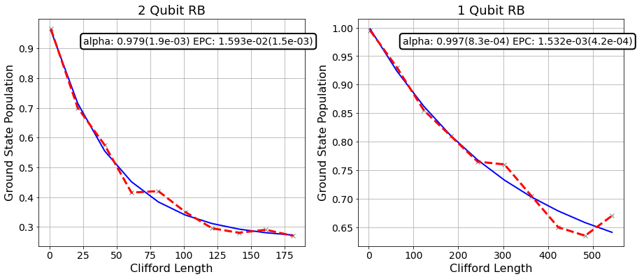
Plot After 1 Seed

plt.figure(figsize=(15, 6))

for i in range(2):
    ax = plt.subplot(1, 2, i+1)
    pattern_ind = i

    # Plot the essence by calling plot_rb_data
    rbfit.plot_rb_data(pattern_ind, ax=ax, add_label=True, show_plt=False)

    # Add title and label
    ax.set_title('%d Qubit RB'%(len(rb_opts['rb_pattern'][i])), fontsize=18)

plt.show()

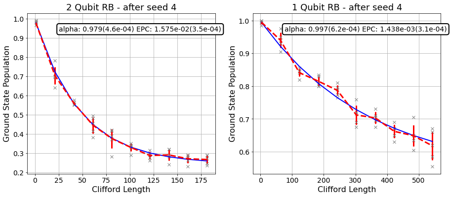
Plot with the Rest of the Seeds

The plot is being updated after each seed.

rbfit = rb.fitters.RBFitter(result_list[0], xdata, rb_opts['rb_pattern'])

for seed_num, data in enumerate(result_list):#range(1,len(result_list)):
    plt.figure(figsize=(15, 6))
    axis = [plt.subplot(1, 2, 1), plt.subplot(1, 2, 2)]

    # Add another seed to the data
    rbfit.add_data([data])

    for i in range(2):
        pattern_ind = i

        # Plot the essence by calling plot_rb_data
        rbfit.plot_rb_data(pattern_ind, ax=axis[i], add_label=True, show_plt=False)

        # Add title and label
        axis[i].set_title('%d Qubit RB - after seed %d'%(len(rb_opts['rb_pattern'][i]), seed_num), fontsize=18)

    # Display
    display.display(plt.gcf())

    # Clear display after each seed and close
    display.clear_output(wait=True)
    time.sleep(1.0)
    plt.close()

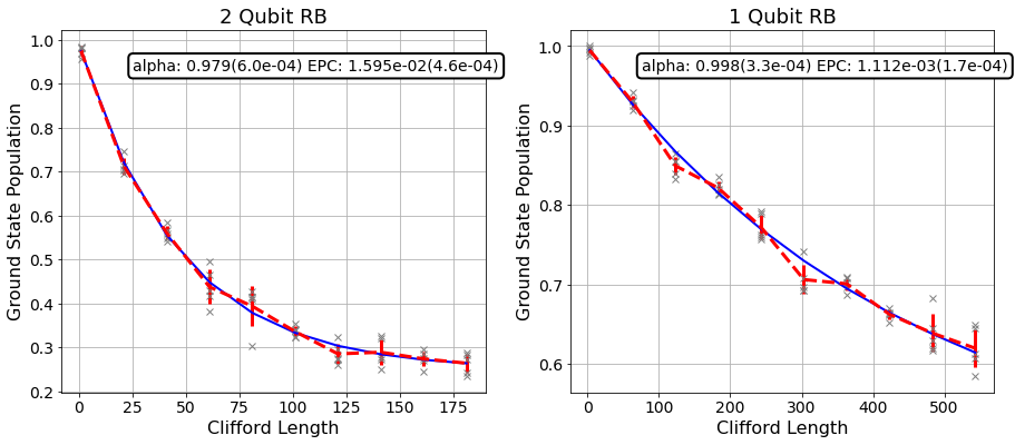
Add more shots to the data

shots = 200
result_list = []
transpile_list = []
for rb_seed,rb_circ_seed in enumerate(rb_circs):
    print('Compiling seed %d'%rb_seed)
    rb_circ_transpile = qiskit.transpile(rb_circ_seed, basis_gates=basis_gates)
    print('Simulating seed %d'%rb_seed)
    job = qiskit.execute(rb_circ_transpile, noise_model=noise_model, shots=shots, backend=backend, backend_options={'max_parallel_experiments': 0})
    result_list.append(job.result())
    transpile_list.append(rb_circ_transpile)
print("Finished Simulating")

Compiling seed 0
Simulating seed 0
Compiling seed 1
Simulating seed 1
Compiling seed 2
Simulating seed 2
Compiling seed 3
Simulating seed 3
Compiling seed 4
Simulating seed 4
Finished Simulating

#Add this data to the previous fit
rbfit.add_data(result_list)

#Replot
plt.figure(figsize=(15, 6))

for i in range(2):
    ax = plt.subplot(1, 2, i+1)
    pattern_ind = i

    # Plot the essence by calling plot_rb_data
    rbfit.plot_rb_data(pattern_ind, ax=ax, add_label=True, show_plt=False)

    # Add title and label
    ax.set_title('%d Qubit RB'%(len(rb_opts['rb_pattern'][i])), fontsize=18)

plt.show()

Predicted Gate Fidelity

From the known depolarizing errors on the simulation we can predict the fidelity. First we need to count the number of gates per Clifford.

The function gates_per_clifford takes a list of transpiled RB circuits and outputs the number of basis gates in each circuit.

#Count the number of single and 2Q gates in the 2Q Cliffords
gates_per_cliff = rb.rb_utils.gates_per_clifford(transpile_list,xdata[0],basis_gates,rb_opts['rb_pattern'][0])
for basis_gate in basis_gates:
    print("Number of %s gates per Clifford: %f "%(basis_gate ,
                                                  np.mean([gates_per_cliff[0][basis_gate],
                                                           gates_per_cliff[2][basis_gate]])))

Number of u1 gates per Clifford: 0.271522
Number of u2 gates per Clifford: 0.923587
Number of u3 gates per Clifford: 0.490109
Number of cx gates per Clifford: 1.526739

The function calculate_2q_epc gives measured errors in the basis gates that were used to construct the Clifford. It assumes that the error in the underlying gates is depolarizing. It outputs the error per a 2-qubit Clifford.

The input to this function is: - gate_per_cliff: dictionary of gate per Clifford. - epg_2q: EPG estimated by error model. - qubit_pair: index of two qubits to calculate EPC. - list_epgs_1q: list of single qubit EPGs of qubit listed in qubit_pair. - two_qubit_name: name of two qubit gate in basis gates (default is cx).

# Error per gate from noise model
epgs_1q = {'u1': 0, 'u2': p1Q/2, 'u3': 2*p1Q/2}
epg_2q = p2Q*3/4
pred_epc = rb.rb_utils.calculate_2q_epc(
    gate_per_cliff=gates_per_cliff,
    epg_2q=epg_2q,
    qubit_pair=[0, 2],
    list_epgs_1q=[epgs_1q, epgs_1q])

# Calculate the predicted epc
print("Predicted 2Q Error per Clifford: %e"%pred_epc)

Predicted 2Q Error per Clifford: 1.591172e-02

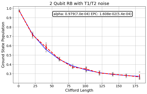
Run an RB Sequence with T1,T2 Errors

We now choose RB sequences that contain only 2-qubit Cliffords.

We execute these sequences as before, but with a noise model extended with T1/T2 thermal relaxation error, and fit the exponentially decaying curve.

rb_opts2 = rb_opts.copy()
rb_opts2['rb_pattern'] = [[0,1]]
rb_opts2['length_multiplier'] = 1
rb_circs2, xdata2 = rb.randomized_benchmarking_seq(**rb_opts2)

noise_model2 = NoiseModel()

#Add T1/T2 noise to the simulation
t1 = 100.
t2 = 80.
gate1Q = 0.1
gate2Q = 0.5
noise_model2.add_all_qubit_quantum_error(thermal_relaxation_error(t1,t2,gate1Q), 'u2')
noise_model2.add_all_qubit_quantum_error(thermal_relaxation_error(t1,t2,2*gate1Q), 'u3')
noise_model2.add_all_qubit_quantum_error(
    thermal_relaxation_error(t1,t2,gate2Q).tensor(thermal_relaxation_error(t1,t2,gate2Q)), 'cx')

backend = qiskit.Aer.get_backend('qasm_simulator')
basis_gates = ['u1','u2','u3','cx'] # use U,CX for now
shots = 500
result_list2 = []
transpile_list2 = []
for rb_seed,rb_circ_seed in enumerate(rb_circs2):
    print('Compiling seed %d'%rb_seed)
    rb_circ_transpile = qiskit.transpile(rb_circ_seed, basis_gates=basis_gates)
    print('Simulating seed %d'%rb_seed)
    job = qiskit.execute(rb_circ_transpile, noise_model=noise_model, shots=shots, backend=backend, backend_options={'max_parallel_experiments': 0})
    result_list2.append(job.result())
    transpile_list2.append(rb_circ_transpile)
print("Finished Simulating")

Compiling seed 0
Simulating seed 0
Compiling seed 1
Simulating seed 1
Compiling seed 2
Simulating seed 2
Compiling seed 3
Simulating seed 3
Compiling seed 4
Simulating seed 4
Finished Simulating

#Create an RBFitter object
rbfit = rb.RBFitter(result_list2, xdata2, rb_opts2['rb_pattern'])

plt.figure(figsize=(10, 6))
ax = plt.gca()

# Plot the essence by calling plot_rb_data
rbfit.plot_rb_data(0, ax=ax, add_label=True, show_plt=False)

# Add title and label
ax.set_title('2 Qubit RB with T1/T2 noise', fontsize=18)

plt.show()

We count again the number of gates per Clifford as before, and calculate the two-qubit Clifford gate error, using the predicted primitive gate errors from the coherence limit.

#Count the number of single and 2Q gates in the 2Q Cliffords
gates_per_cliff = rb.rb_utils.gates_per_clifford(transpile_list2,xdata[0],basis_gates,rb_opts2['rb_pattern'][0])
for basis_gate in basis_gates:
    print("Number of %s gates per Clifford: %f "%(basis_gate ,
                                                  np.mean([gates_per_cliff[0][basis_gate],
                                                           gates_per_cliff[1][basis_gate]])))

Number of u1 gates per Clifford: 0.250761
Number of u2 gates per Clifford: 0.969565
Number of u3 gates per Clifford: 0.489130
Number of cx gates per Clifford: 1.503696

# Predicted primitive gate errors from the coherence limit
u2_error = rb.rb_utils.coherence_limit(1,[t1],[t2],gate1Q)
u3_error = rb.rb_utils.coherence_limit(1,[t1],[t2],2*gate1Q)
epg_2q = rb.rb_utils.coherence_limit(2,[t1,t1],[t2,t2],gate2Q)
epgs_1q = {'u1': 0, 'u2': u2_error, 'u3': u3_error}
pred_epc = rb.rb_utils.calculate_2q_epc(
    gate_per_cliff=gates_per_cliff,
    epg_2q=epg_2q,
    qubit_pair=[0, 1],
    list_epgs_1q=[epgs_1q, epgs_1q])

# Calculate the predicted epc
print("Predicted 2Q Error per Clifford: %e"%pred_epc)

Predicted 2Q Error per Clifford: 1.313111e-02

import qiskit.tools.jupyter
%qiskit_version_table
%qiskit_copyright

Version Information

Qiskit Software	Version
Qiskit	0.16.1
Terra	0.13.0.dev0+98fd14e
Aer	0.4.1
Ignis	0.3.0.dev0+dd2c926
Aqua	0.6.4
IBM Q Provider	0.5.0
System information
Python	3.7.6 (default, Jan 8 2020, 19:59:22) [GCC 7.3.0]
OS	Linux
CPUs	8
Memory (Gb)	62.920127868652344
Fri Mar 27 15:44:43 2020 IST

This code is a part of Qiskit

© Copyright IBM 2017, 2020.

This code is licensed under the Apache License, Version 2.0. You may
obtain a copy of this license in the LICENSE.txt file in the root directory
of this source tree or at http://www.apache.org/licenses/LICENSE-2.0.

Any modifications or derivative works of this code must retain this
copyright notice, and modified files need to carry a notice indicating
that they have been altered from the originals.