Note
This page was generated from tutorials/simulators/1_aer_provider.ipynb.
Simulators
Introduction
This notebook shows how to import the Qiskit Aer simulator backend and use it to run ideal (noise free) Qiskit Terra circuits.
[1]:
import numpy as np

# Import Qiskit
from qiskit import QuantumCircuit
from qiskit import Aer, transpile
from qiskit.tools.visualization import plot_histogram, plot_state_city
import qiskit.quantum_info as qi
The Aer Provider
The Aer provider contains a variety of high performance simulator backends for a variety of simulation methods. The available backends on the current system can be viewed using Aer.backends
[2]:
Aer.backends()
[2]:
[AerSimulator('aer_simulator'),
 AerSimulator('aer_simulator_statevector'),
 AerSimulator('aer_simulator_density_matrix'),
 AerSimulator('aer_simulator_stabilizer'),
 AerSimulator('aer_simulator_matrix_product_state'),
 AerSimulator('aer_simulator_extended_stabilizer'),
 AerSimulator('aer_simulator_unitary'),
 AerSimulator('aer_simulator_superop'),
 QasmSimulator('qasm_simulator'),
 StatevectorSimulator('statevector_simulator'),
 UnitarySimulator('unitary_simulator'),
 PulseSimulator('pulse_simulator')]
The Aer Simulator
The main simulator backend of the Aer provider is the AerSimulator backend. A new simulator backend can be created using Aer.get_backend('aer_simulator').
[3]:
simulator = Aer.get_backend('aer_simulator')
The default behavior of the AerSimulator backend is to mimic the execution of an actual device. If a QuantumCircuit containing measurements is run it will return a count dictionary containing the final values of any classical registers in the circuit. The circuit may contain gates, measurements, resets, conditionals, and other custom simulator instructions that will be discussed in another notebook.
Simulating a quantum circuit
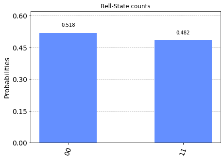
The basic operation runs a quantum circuit and returns a counts dictionary of measurement outcomes. Here we run a simple circuit that prepares a 2-qubit Bell-state \(\left|\psi\right\rangle = \frac{1}{2}\left(\left|0,0\right\rangle + \left|1,1 \right\rangle\right)\) and measures both qubits.
[4]:
# Create circuit
circ = QuantumCircuit(2)
circ.h(0)
circ.cx(0, 1)
circ.measure_all()

# Transpile for simulator
simulator = Aer.get_backend('aer_simulator')
circ = transpile(circ, simulator)

# Run and get counts
result = simulator.run(circ).result()
counts = result.get_counts(circ)
plot_histogram(counts, title='Bell-State counts')
[4]:
Returning measurement outcomes for each shot
The QasmSimulator also supports returning a list of measurement outcomes for each individual shot. This is enabled by setting the keyword argument memory=True in the run.
[5]:
# Run and get memory
result = simulator.run(circ, shots=10, memory=True).result()
memory = result.get_memory(circ)
print(memory)
['11', '00', '00', '11', '00', '11', '00', '00', '11', '00']
Aer Simulator Options
The AerSimulator backend supports a variety of configurable options which can be updated using the set_options method. See the AerSimulator API documentation for additional details.
Simulation Method
The AerSimulator supports a variety of simulation methods, each of which supports a different set of instructions. The method can be set manually using simulator.set_option(method=value) option, or a simulator backend with a preconfigured method can be obtained directly from the Aer provider using Aer.get_backend.
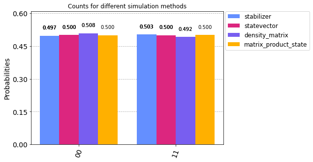
When simulating ideal circuits, changing the method between the exact simulation methods stabilizer, statevector, density_matrix and matrix_product_state should not change the simulation result (other than usual variations from sampling probabilities for measurement outcomes)
[6]:
# Increase shots to reduce sampling variance
shots = 10000

# Stabilizer simulation method
sim_stabilizer = Aer.get_backend('aer_simulator_stabilizer')
job_stabilizer = sim_stabilizer.run(circ, shots=shots)
counts_stabilizer = job_stabilizer.result().get_counts(0)

# Statevector simulation method
sim_statevector = Aer.get_backend('aer_simulator_statevector')
job_statevector = sim_statevector.run(circ, shots=shots)
counts_statevector = job_statevector.result().get_counts(0)

# Density Matrix simulation method
sim_density = Aer.get_backend('aer_simulator_density_matrix')
job_density = sim_density.run(circ, shots=shots)
counts_density = job_density.result().get_counts(0)

# Matrix Product State simulation method
sim_mps = Aer.get_backend('aer_simulator_matrix_product_state')
job_mps = sim_mps.run(circ, shots=shots)
counts_mps = job_mps.result().get_counts(0)

plot_histogram([counts_stabilizer, counts_statevector, counts_density, counts_mps],
               title='Counts for different simulation methods',
               legend=['stabilizer', 'statevector',
                       'density_matrix', 'matrix_product_state'])
[6]:
Automatic Simulation Method
The default simulation method is automatic which will automatically select a one of the other simulation methods for each circuit based on the instructions in those circuits. A fixed simulation method can be specified by by adding the method name when getting the backend, or by setting the method option on the backend.
GPU Simulation
The statevector, density_matrix and unitary simulators support running on a NVidia GPUs. For these methods the simulation device can also be manually set to CPU or GPU using simulator.set_options(device='GPU') backend option. If a GPU device is not available setting this option will raise an exception.
[7]:
from qiskit.providers.aer import AerError

# Initialize a GPU backend
# Note that the cloud instance for tutorials does not have a GPU
# so this will raise an exception.
try:
    simulator_gpu = Aer.get_backend('aer_simulator')
    simulator_gpu.set_options(device='GPU')
except AerError as e:
    print(e)
"Invalid simulation device GPU. Available devices are: ['CPU']"
The Aer provider will also contain preconfigured GPU simulator backends if Qiskit Aer was installed with GPU support on a compatible system:
aer_simulator_statevector_gpuaer_simulator_density_matrix_gpuaer_simulator_unitary_gpu
Note: The GPU version of Aer can be installed using ``pip install qiskit-aer-gpu``.
Simulation Precision
One of the available simulator options allows setting the float precision for the statevector, density_matrix unitary and superop methods. This is done using the set_precision="single" or precision="double" (default) option:
[8]:
# Configure a single-precision statevector simulator backend
simulator = Aer.get_backend('aer_simulator_statevector')
simulator.set_options(precision='single')

# Run and get counts
result = simulator.run(circ).result()
counts = result.get_counts(circ)
print(counts)
{'11': 503, '00': 521}
Setting the simulation precision applies to both CPU and GPU simulation devices. Single precision will halve the required memory and may provide performance improvements on certain systems.
Custom Simulator Instructions
Saving the simulator state
The state of the simulator can be saved in a variety of formats using custom simulator instructions.
Circuit method |
Description |
Supported Methods |
|---|---|---|
|
Save the simulator state in the native format for the simulation method |
All |
|
Save the simulator state as a statevector |
|
|
Save the simulator state as a Clifford stabilizer |
|
|
Save the simulator state as a density matrix |
|
|
Save the simulator state as a a matrix product state tensor |
|
|
Save the simulator state as unitary matrix of the run circuit |
|
|
Save the simulator state as superoperator matrix of the run circuit |
|
Note that these instructions are only supported by the Aer simulator and will result in an error if a circuit containing them is run on a non-simulator backend such as an IBM Quantum device.
Saving the final statevector
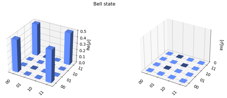
To save the final statevector of the simulation we can append the circuit with the save_statevector instruction. Note that this instruction should be applied before any measurements if we do not want to save the collapsed post-measurement state
[9]:
# Construct quantum circuit without measure
circ = QuantumCircuit(2)
circ.h(0)
circ.cx(0, 1)
circ.save_statevector()

# Transpile for simulator
simulator = Aer.get_backend('aer_simulator')
circ = transpile(circ, simulator)

# Run and get statevector
result = simulator.run(circ).result()
statevector = result.get_statevector(circ)
plot_state_city(statevector, title='Bell state')
[9]:
Saving the circuit unitary
To save the unitary matrix for a QuantumCircuit we can append the circuit with the save_unitary instruction. Note that this circuit cannot contain any measurements or resets since these instructions are not supported on for the "unitary" simulation method
[10]:
# Construct quantum circuit without measure
circ = QuantumCircuit(2)
circ.h(0)
circ.cx(0, 1)
circ.save_unitary()

# Transpile for simulator
simulator = Aer.get_backend('aer_simulator')
circ = transpile(circ, simulator)

# Run and get unitary
result = simulator.run(circ).result()
unitary = result.get_unitary(circ)
print("Circuit unitary:\n", unitary.round(5))
Circuit unitary:
 [[ 0.70711+0.j  0.70711-0.j  0.     +0.j  0.     +0.j]
 [ 0.     +0.j  0.     +0.j  0.70711+0.j -0.70711+0.j]
 [ 0.     +0.j  0.     +0.j  0.70711+0.j  0.70711-0.j]
 [ 0.70711+0.j -0.70711+0.j  0.     +0.j  0.     +0.j]]
Saving multiple states
We can also apply save instructions at multiple locations in a circuit. Note that when doing this we must provide a unique label for each instruction to retrieve them from the results
[11]:
# Construct quantum circuit without measure
steps = 5
circ = QuantumCircuit(1)
for i in range(steps):
    circ.save_statevector(label=f'psi_{i}')
    circ.rx(i * np.pi / steps, 0)
circ.save_statevector(label=f'psi_{steps}')

# Transpile for simulator
simulator = Aer.get_backend('aer_simulator')
circ = transpile(circ, simulator)

# Run and get saved data
result = simulator.run(circ).result()
data = result.data(0)
data
[11]:
{'psi_5': array([-1.+0.00000000e+00j,  0.-5.55111512e-17j]),
 'psi_3': array([0.58778525+0.j        , 0.        -0.80901699j]),
 'psi_2': array([0.95105652+0.j        , 0.        -0.30901699j]),
 'psi_0': array([1.+0.j, 0.+0.j]),
 'psi_4': array([-0.30901699+0.j        ,  0.        -0.95105652j]),
 'psi_1': array([1.+0.j, 0.+0.j])}
Setting the simulator to a custom state
The AerSimulator allows setting a custom simulator state for several of its simulation methods using custom simulator instructions
Circuit method |
Description |
Supported Methods |
|---|---|---|
|
Set the simulator state to the specified statevector |
|
|
Set the simulator state to the specified Clifford stabilizer |
|
|
Set the simulator state to the specified density matrix |
|
|
Set the simulator state to the specified unitary matrix |
|
|
Set the simulator state to the specified superoperator matrix |
|
Notes: * These instructions must be applied to all qubits in a circuit, otherwise an exception will be raised. * The input state must also be a valid state (statevector, density matrix, unitary etc) otherwise an exception will be raised. * These instructions can be applied at any location in a circuit and will override the current state with the specified one. Any classical register values (e.g. from preceding measurements) will be unaffected * Set state instructions are only supported by the Aer simulator and will result in an error if a circuit containing them is run on a non-simulator backend such as an IBM Quantum device.
Setting a custom statevector
The set_statevector instruction can be used to set a custom Statevector state. The input statevector must be valid (\(|\langle\psi|\psi\rangle|=1\))
[12]:
# Generate a random statevector
num_qubits = 2
psi = qi.random_statevector(2 ** num_qubits, seed=100)

# Set initial state to generated statevector
circ = QuantumCircuit(num_qubits)
circ.set_statevector(psi)
circ.save_state()

# Transpile for simulator
simulator = Aer.get_backend('aer_simulator')
circ = transpile(circ, simulator)

# Run and get saved data
result = simulator.run(circ).result()
result.data(0)
[12]:
{'statevector': array([ 0.18572453-0.03102771j, -0.26191269-0.18155865j,
         0.12367038-0.47837907j,  0.66510011-0.4200986j ])}
Using the initialize instruction
It is also possible to initialize the simulator to a custom statevector using the initialize instruction. Unlike the set_statevector instruction this instruction is also supported on real device backends by unrolling to reset and standard gate instructions.
[13]:
# Use initilize instruction to set initial state
circ = QuantumCircuit(num_qubits)
circ.initialize(psi, range(num_qubits))
circ.save_state()

# Transpile for simulator
simulator = Aer.get_backend('aer_simulator')
circ = transpile(circ, simulator)

# Run and get result data
result = simulator.run(circ).result()
result.data(0)
[13]:
{'statevector': array([ 0.18572453-0.03102771j, -0.26191269-0.18155865j,
         0.12367038-0.47837907j,  0.66510011-0.4200986j ])}
Setting a custom density matrix
The set_density_matrix instruction can be used to set a custom DensityMatrix state. The input density matrix must be valid (\(Tr[\rho]=1, \rho \ge 0\))
[14]:
num_qubits = 2
rho = qi.random_density_matrix(2 ** num_qubits, seed=100)
circ = QuantumCircuit(num_qubits)
circ.set_density_matrix(rho)
circ.save_state()

# Transpile for simulator
simulator = Aer.get_backend('aer_simulator')
circ = transpile(circ, simulator)

# Run and get saved data
result = simulator.run(circ).result()
result.data(0)
[14]:
{'density_matrix': array([[ 0.2075308 +0.j        ,  0.13161422-0.01760848j,
          0.0442826 +0.07742704j,  0.04852053-0.01303171j],
        [ 0.13161422+0.01760848j,  0.20106116+0.j        ,
          0.02568549-0.03689812j,  0.0482903 -0.04367912j],
        [ 0.0442826 -0.07742704j,  0.02568549+0.03689812j,
          0.39731492+0.j        , -0.01114025-0.13426423j],
        [ 0.04852053+0.01303171j,  0.0482903 +0.04367912j,
         -0.01114025+0.13426423j,  0.19409312+0.j        ]])}
Setting a custom stabilizer state
The set_stabilizer instruction can be used to set a custom Clifford stabilizer state. The input stabilizer must be a valid Clifford.
[15]:
# Generate a random Clifford C
num_qubits = 2
stab = qi.random_clifford(num_qubits, seed=100)

# Set initial state to stabilizer state C|0>
circ = QuantumCircuit(num_qubits)
circ.set_stabilizer(stab)
circ.save_state()

# Transpile for simulator
simulator = Aer.get_backend('aer_simulator')
circ = transpile(circ, simulator)

# Run and get saved data
result = simulator.run(circ).result()
result.data(0)
[15]:
{'stabilizer': {'destabilizer': ['-XZ', '-YX'], 'stabilizer': ['+ZZ', '-IZ']}}
Setting a custom unitary
The set_unitary instruction can be used to set a custom unitary Operator state. The input unitary matrix must be valid (\(U^\dagger U=\mathbb{1}\))
[16]:
# Generate a random unitary
num_qubits = 2
unitary = qi.random_unitary(2 ** num_qubits, seed=100)

# Set initial state to unitary
circ = QuantumCircuit(num_qubits)
circ.set_unitary(unitary)
circ.save_state()

# Transpile for simulator
simulator = Aer.get_backend('aer_simulator')
circ = transpile(circ, simulator)

# Run and get saved data
result = simulator.run(circ).result()
result.data(0)
[16]:
{'unitary': array([[-0.44885724-0.26721573j,  0.10468034-0.00288681j,
          0.4631425 +0.15474915j, -0.11151309-0.68210936j],
        [-0.37279054-0.38484834j,  0.3820592 -0.49653433j,
          0.14132327-0.17428515j,  0.19643043+0.48111423j],
        [ 0.2889092 +0.58750499j,  0.39509694-0.22036424j,
          0.49498355+0.2388685j ,  0.25404989-0.00995706j],
        [ 0.01830684+0.10524311j,  0.62584001+0.01343146j,
         -0.52174025-0.37003296j,  0.12232823-0.41548904j]])}
[17]:
import qiskit.tools.jupyter
%qiskit_version_table
%qiskit_copyright
/home/computertreker/git/qiskit/qiskit/.tox/docs/lib/python3.7/site-packages/qiskit/aqua/__init__.py:86: DeprecationWarning: The package qiskit.aqua is deprecated. It was moved/refactored to qiskit-terra For more information see <https://github.com/Qiskit/qiskit-aqua/blob/main/README.md#migration-guide>
  warn_package('aqua', 'qiskit-terra')
Version Information
| Qiskit Software | Version |
|---|---|
qiskit-terra | 0.18.2 |
qiskit-aer | 0.8.2 |
qiskit-ignis | 0.6.0 |
qiskit-ibmq-provider | 0.16.0 |
qiskit-aqua | 0.9.5 |
qiskit | 0.29.1 |
qiskit-nature | 0.2.2 |
qiskit-finance | 0.3.0 |
qiskit-optimization | 0.2.3 |
qiskit-machine-learning | 0.2.1 |
| System information | |
| Python | 3.7.12 (default, Nov 22 2021, 14:57:10) [GCC 11.1.0] |
| OS | Linux |
| CPUs | 32 |
| Memory (Gb) | 125.71650314331055 |
| Tue Jan 04 11:17:52 2022 EST | |
This code is a part of Qiskit
© Copyright IBM 2017, 2022.
This code is licensed under the Apache License, Version 2.0. You may
obtain a copy of this license in the LICENSE.txt file in the root directory
of this source tree or at http://www.apache.org/licenses/LICENSE-2.0.
Any modifications or derivative works of this code must retain this
copyright notice, and modified files need to carry a notice indicating
that they have been altered from the originals.