Note

This page was generated from tutorials/noise/9_entanglement_verification.ipynb.

Entanglement Verification

Introduction to the GHZ state

The Greenberger-Horne-Zeilinger (GHZ) State is a \(n\)-qubit entangled state best defined by the following state vector:

\[|{\rm GHZ} \rangle = \frac{|0 \rangle ^{\otimes n} + |1 \rangle ^{\otimes n}}{\sqrt{2}} , n > 2\]

Characterization of the GHZ state is very useful in assessing multi-qubit interactions, whose robustness is key to developing large scale quantum computers.

Characterizing a quantum state

Any mixed quantum state can be identified by a density matrix, defined as \(\rho = \sum_{i} p_i |\psi_{i} \rangle \langle \psi_{i}|\), where \(|\psi_{i} \rangle\) are the pure quantum states forming the mixture and \(0 < p_i \le 1\), \(\sum_{i} p_i = 1\) are the classical probabilities to be in state \(|\psi_{i} \rangle\). We denote the pure density matrix of an ideal GHZ State by \(\rho_{p} \equiv |{\rm GHZ} \rangle \langle {\rm GHZ}|\). We want to see how close this matrix is to the density matrix of a GHZ State as produced in an experiment, \(\rho_{T}\). One method to quantify this similarity is to calculate the fidelity between the states, \(F(\rho_{p},\rho_{T})\)

\[F = \Big[ Tr \sqrt{\sqrt{\rho_{p}}\rho_{T}\sqrt{\rho_{p}}} \Big] ^{2}\]

The aim of this tutorial is two-fold: we will explore ways in which we can characterize the GHZ state, and ways in which we can use Ignis’ error mitigation tools to increase readout fidelity, regardless of characterization method

Before we go further, let us import everything we will need from basic Qiskit:

from qiskit import IBMQ, execute
from qiskit import Aer
from qiskit import QuantumRegister
from qiskit.tools.monitor import job_monitor
from qiskit.circuit import Parameter
from qiskit.providers.aer import noise
from qiskit import quantum_info
from qiskit import visualization

import numpy as np
import matplotlib.pyplot as plt

The next two functions are from ignis. The first is for the general error mitigation technique, and the second is specifically for quantum tomography

from qiskit.ignis.mitigation.measurement import (complete_meas_cal, tensored_meas_cal,
                                                 CompleteMeasFitter, TensoredMeasFitter)
from qiskit.ignis.verification.tomography import state_tomography_circuits, StateTomographyFitter

The following import from the entanglement package contains information needed to create, parallelize and analyze GHZ State circuits

from qiskit.ignis.verification.entanglement.parallelize import *
from qiskit.ignis.verification.entanglement.linear import *
from qiskit.ignis.verification.entanglement.analysis import Plotter

Preparing a GHZ State

Let us first go over how to prepare a GHZ State:

Say we have a system of \(n\) qubits, all prepared in the \(|0\rangle\) state:

\[|\psi \rangle = |00...0\rangle\]

We apply a Hadamard gate to the first qubit: \(|0\rangle \longrightarrow \frac{1}{\sqrt{2}}(|0\rangle + |1\rangle)\). Our state now looks like:

\[|\psi \rangle = \frac{|00...0\rangle + |10...0\rangle}{\sqrt{2}}\]

Applying on this state a sequence of \(n-1\) CNOT gate between the \(n^{th}\) and \((n+1)^{th}\) qubits for \(n = 0 \ldots n-1\) leaves the \(n+1\) qubit at \(|0\rangle\) if the \(n^{th}\) is in \(|0\rangle\), and at \(|1\rangle\) if the \(n^{th}\) is in \(|1\rangle\), thus creating the GHZ State:

\[|GHZ \rangle = \frac{|00...0\rangle + |11...1\rangle}{\sqrt{2}} \equiv \frac{|0 \rangle ^{\otimes n} + |1 \rangle ^{\otimes n}}{\sqrt{2}}\]

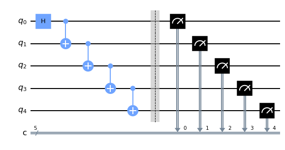
The following function creates this “linear” circuit that can measure the GHZ state:

qn = 5 #creating a 5 qubit GHZ state
circ_simple = get_ghz_simple(qn,measure=True)

/home/computertreker/git/qiskit/qiskit/.tox/docs/lib/python3.7/site-packages/qiskit/ignis/verification/entanglement/linear.py:84: DeprecationWarning: The QuantumCircuit.__add__() method is being deprecated.Use the compose() method which is more flexible w.r.t circuit register compatibility.
  circ = circ + meas
/home/computertreker/git/qiskit/qiskit/.tox/docs/lib/python3.7/site-packages/qiskit/circuit/quantumcircuit.py:933: DeprecationWarning: The QuantumCircuit.combine() method is being deprecated. Use the compose() method which is more flexible w.r.t circuit register compatibility.
  return self.combine(rhs)

circ_simple.draw(output='mpl')

Characterization, Part I

Multiple Quantum Coherence (MQC)

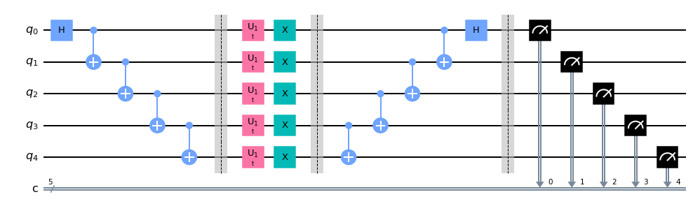
Multiple Quantum Coherence (MQC) works by taking the preliminary preparation of an \(n\) qubit GHZ State, and rotating each of the qubit states around the z axis by a phase \(\phi\). After that, we apply a X gate, i.e., a \(\pi\) pulse around the x axis. Then, we apply the inverse of the operations we originally applied to get the GHZ state. In an ideal situation the final state is \(|\psi \rangle = \frac{|0 \rangle ^{\otimes n} + e^{i n \phi}|1 \rangle ^{\otimes n}}{\sqrt{2}}\). We can ideally observe the phase collected by projecting \(|\psi \rangle\) onto the state \(|0 \rangle ^{\otimes n}\). This technique is reminiscent of an echo sequence, and has been shown to substantially improve the fidelity during readout.

The function below creates a linear MQC circuit. As with every circuit from here on, you can change the full_measurement argument to toggle between full measurement of all qubits or measurement of only the control qubit. Full measurement yields the most accurate results, but for more than 7 qubits, it is recommended to set it to false, and observe only the oscillations between the '0' and '1' states.

circ_mqc = get_ghz_mqc_para(qn, full_measurement=True)

/home/computertreker/git/qiskit/qiskit/.tox/docs/lib/python3.7/site-packages/qiskit/ignis/verification/entanglement/linear.py:142: DeprecationWarning: The QuantumCircuit.__iadd__() method is being deprecated. Use the compose() (potentially with the inplace=True argument) and tensor() methods which are more flexible w.r.t circuit register compatibility.
  circ += circinv
/home/computertreker/git/qiskit/qiskit/.tox/docs/lib/python3.7/site-packages/qiskit/circuit/quantumcircuit.py:942: DeprecationWarning: The QuantumCircuit.extend() method is being deprecated. Use the compose() (potentially with the inplace=True argument) and tensor() methods which are more flexible w.r.t circuit register compatibility.
  return self.extend(rhs)

circ_mqc[0].draw(output='mpl')

/home/computertreker/git/qiskit/qiskit/.tox/docs/lib/python3.7/site-packages/sympy/core/expr.py:3951: SymPyDeprecationWarning:

expr_free_symbols method has been deprecated since SymPy 1.9. See
https://github.com/sympy/sympy/issues/21494 for more info.

  deprecated_since_version="1.9").warn()

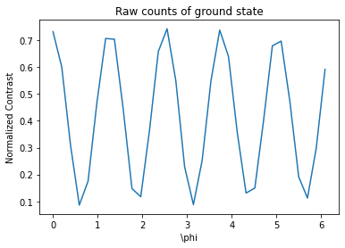
After running experiments on this MQC circuit, we can pick a state to observe oscillations as we sweep \(\phi\) from \(0\) to \(2 \pi\). Our signal in theory should follow \(S(\phi) = \frac{1}{2}(1+\cos(n \phi))\). We then perform a Discrete Fourier Transform (DFT: \(I_{v}=(1/N)|\sum_{\phi}e^{iv\phi}S(\phi)\)) to extract the Fidelity of the state, defined by the bounds \(2\sqrt{I_{n}} \leq F \leq \sqrt{I_{0}/2}+ \sqrt{I_{n}}\); if desired, an actual value for the fidelity can be obtained: \(F = \frac{1}{2}(P_{00...0}+P_{11...1})+\sqrt{I_{n}})\) (arXiv:1905.05720).

Parity Oscillations

The next method we use to characterize the GHZ state is parity oscillations. After preparing a GHZ state, we apply a combination of rotations about the x and y axes to create various superposition states as a function of \(\phi\): \(U(\phi) = \otimes_{j}^{N} e^{i\frac{\pi}{4}(\cos(\phi)\sigma_{x}^{j}+\sin(\phi)\sigma_{y}^{j})}\). We then measure the expectation value \(\langle \otimes_{j}^{N} \sigma_{z}^{j} \rangle_{\phi}\) as a function of \(\phi\), which in theory should lead to parity oscillations between 1 and -1.

The following function generates a circuit which is the Parity Oscillation equivalent of the MQC circuit given above

circ_po = get_ghz_po_para(qn)

circ_po[0].draw(output='mpl')

We can obtain fidelity for parity oscillations \(S_{\phi}\) from \(F = \frac{1}{2}(P_{00...0}+P_{11...1}+C)\), where \(C\), the coherence is defined as \(2\sqrt{I_{n}}\), following the same convention for the DFT as with the MQC method.

Tomography

Tomography measures the density matrix by producing many nominally identical states and measuring the state instances in different bases. The ideal result of a GHZ state is four equal density matrix elements at the 4 corners of the tensor-product basis, with all other elements vanishing. Although the fidelity can be readily calculated by this method, the method is slow (requires exponential number of measurements in n), and takes prohibitively long times if n is larger than 7 or so. Nevertheless, we will show below how to perform this method as it is relevant for small numbers of qubits.

Parallelizing circuits

The above “linear” circuits are good to perform simulations, but what do we do when we use real devices, where the system can have an arbitrary topology and various errors? We are specifically targeting real hardware here, not just Aer simulation. One technique to reduce real-hardware effects is to parallelize the CNOT gates and thus create a shorter-depth circuit. This can be hugely beneficial efficiency wise, and fidelity wise. The class BConfig from the module parallelize does exactly this.

First we must configure the optimal backend we want to use. We will consider a simulation backend, 'ibmq_qasm_simulator', disguised as a real device, 'ibmq_16_melbourne' by using a the mock backend 'FakeMelbourne'

from qiskit.providers.aer import QasmSimulator
from qiskit.test.mock import FakeMelbourne
backend = QasmSimulator()
backend_hardware = FakeMelbourne()

Using the noise module, we can now define a noise model from 'ibmq_16_melbourne' to “assign” to 'ibmq_qasm_simulator'.

noise_model = noise.NoiseModel.from_backend(backend_hardware)
coupling_map = backend_hardware._configuration.coupling_map
basis_gates=noise_model.basis_gates

And there we have it. From now on, in the tutorial, when using a real device, not a simulation, just take out every mention and assignment of noise_model and coupling_map, and assign the real device to backend. The simulator used from now on is no substitute for running a real device.

BConfig lays the blueprint for creating parallelized circuits. Let us initialize an object taking in the real device we just defined, and name it protocirc. All of our experiments will use it:

protocirc = BConfig(backend_hardware)

Error Mitigation

Qiskit Ignis provides very accurate tools to take raw data and return calibrated data. This is done by getting the raw data, in the form of a vector \(v_{raw}\) and getting a calibration matrix \(A\). The output is then the solution to the optimization problem: \(argmin_{v_{cal}} ||Av_{cal}-v_{raw}||^{2}\)

Experiment Time

Preliminary Steps

The probabilities of measuring \(|0\rangle ^{\otimes n}\) and \(|1\rangle^{\otimes n}\) in the GHZ state are important in calculating fidelity. For this, we need to run the following test

We begin by defining standard execution parameters:

shots = 1024 #numbers of shots in a given experiment
max_credits = 3 #number of credits
qn = 5 #number of qubits
zerocode = '0'*qn #will help us easily define the state |00...00>
onecode = '1'*qn #will help us easily define the state |11...11>
sweep = np.arange(0.,np.pi*2,np.pi/16) #standard list of phase values we will sweep

circ_simple, qr, initial_layout = protocirc.get_ghz_simple(qn, True)

print(initial_layout)
circ_simple.draw()

{Qubit(QuantumRegister(5, 'q'), 0): 1, Qubit(QuantumRegister(5, 'q'), 1): 2, Qubit(QuantumRegister(5, 'q'), 2): 0, Qubit(QuantumRegister(5, 'q'), 3): 3, Qubit(QuantumRegister(5, 'q'), 4): 13}

                       ░ ┌───┐ ░                               ░  ░       ┌─┐»
 q_0: ─────────────────░─┤ X ├─░───────────────────────────────░──░───────┤M├»
      ┌─────────┐      ░ └─┬─┘ ░ ┌──────────┐┌───┐┌──────────┐ ░  ░ ┌─┐   └╥┘»
 q_1: ┤ U2(0,π) ├──■───░───■───░─┤ U2(0,-π) ├┤ X ├┤ U2(0,-π) ├─░──░─┤M├────╫─»
      └─────────┘┌─┴─┐ ░       ░ └──────────┘└─┬─┘└──────────┘ ░  ░ └╥┘┌─┐ ║ »
 q_2: ───────────┤ X ├─░───■───░───────────────┼───────────────░──░──╫─┤M├─╫─»
                 └───┘ ░ ┌─┴─┐ ░               │               ░  ░  ║ └╥┘ ║ »
 q_3: ─────────────────░─┤ X ├─░───────────────┼───────────────░──░──╫──╫──╫─»
                       ░ └───┘ ░               │               ░  ░  ║  ║  ║ »
 q_4: ─────────────────────────────────────────┼─────────────────────╫──╫──╫─»
                                               │                     ║  ║  ║ »
 q_5: ─────────────────────────────────────────┼─────────────────────╫──╫──╫─»
                                               │                     ║  ║  ║ »
 q_6: ─────────────────────────────────────────┼─────────────────────╫──╫──╫─»
                                               │                     ║  ║  ║ »
 q_7: ─────────────────────────────────────────┼─────────────────────╫──╫──╫─»
                                               │                     ║  ║  ║ »
 q_8: ─────────────────────────────────────────┼─────────────────────╫──╫──╫─»
                                               │                     ║  ║  ║ »
 q_9: ─────────────────────────────────────────┼─────────────────────╫──╫──╫─»
                                               │                     ║  ║  ║ »
q_10: ─────────────────────────────────────────┼─────────────────────╫──╫──╫─»
                                               │                     ║  ║  ║ »
q_11: ─────────────────────────────────────────┼─────────────────────╫──╫──╫─»
                                               │                     ║  ║  ║ »
q_12: ─────────────────────────────────────────┼─────────────────────╫──╫──╫─»
                       ░       ░ ┌──────────┐  │  ┌──────────┐ ░  ░  ║  ║  ║ »
q_13: ─────────────────░───────░─┤ U2(0,-π) ├──■──┤ U2(0,-π) ├─░──░──╫──╫──╫─»
                       ░       ░ └──────────┘     └──────────┘ ░  ░  ║  ║  ║ »
 c: 5/═══════════════════════════════════════════════════════════════╩══╩══╩═»
                                                                     0  1  2 »
«
« q_0: ──────
«
« q_1: ──────
«
« q_2: ──────
«      ┌─┐
« q_3: ┤M├───
«      └╥┘
« q_4: ─╫────
«       ║
« q_5: ─╫────
«       ║
« q_6: ─╫────
«       ║
« q_7: ─╫────
«       ║
« q_8: ─╫────
«       ║
« q_9: ─╫────
«       ║
«q_10: ─╫────
«       ║
«q_11: ─╫────
«       ║
«q_12: ─╫────
«       ║ ┌─┐
«q_13: ─╫─┤M├
«       ║ └╥┘
« c: 5/═╩══╩═
«       3  4 

job_simple = execute(circ_simple, backend, shots=shots, max_credits=max_credits,noise_model=noise_model)
# job_simple = execute(circ_simple, backend, shots=shots, max_credits=max_credits,noise_model=noise_model, coupling_map=coupling_map, basis_gates=basis_gates)

job_monitor(job_simple)
result_simple = job_simple.result()

Job Status: job has successfully run

P0 = (1/shots)*result_simple.get_counts()[zerocode]
P1 = (1/shots)*result_simple.get_counts()[onecode]
print('P(|00...0>) = ',P0)
print('P(|11...1>) = ',P1)

P(|00...0>) =  0.41796875
P(|11...1>) =  0.3125

Now with error mitigation:

qr = QuantumRegister(qn)
qubit_list = range(qn)
meas_calibs_simple, state_labels_simple = complete_meas_cal(qubit_list=qubit_list, qr=qr, circlabel='mcal')

job_simple_em = execute(meas_calibs_simple, backend=backend,
                     noise_model=noise_model)
job_monitor(job_simple_em)
meas_result = job_simple_em.result()

Job Status: job has successfully run

meas_fitter = CompleteMeasFitter(meas_result,state_labels_simple,circlabel='mcal')
result_simple_em = meas_fitter.filter.apply(result_simple)

result_simple_em.get_counts()[zerocode]*1/shots

0.4549262956373367

P0_m = (1/shots)*result_simple_em.get_counts()[zerocode]
P1_m = (1/shots)*result_simple_em.get_counts()[onecode]
print('P(|00...0>) error mitigated = ',P0_m)
print('P(|11...1>) error mitigated = ',P1_m)

P(|00...0>) error mitigated =  0.4549262956373367
P(|11...1>) error mitigated =  0.427516659876316

We will load these values in a dictionary for assessing fidelity later on:

p_dict = {'P0': P0, 'P1': P1, 'P0_m': P0_m, 'P1_m':P1_m}

Part 1 : MQC

We now retrieve a parallelized MQC circuit for the n qubit device

shots = 1024 #numbers of shots in a given experiment
max_credits = 3 #number of credits
qn = 5 #number of qubits
zerocode = '0'*qn #will help us easily define the state |00...00>
sweep = np.arange(0.,np.pi*2,np.pi/16) #standard list of phase values we will sweep

%%time
circ, theta,initial_layout = protocirc.get_ghz_mqc_para(qn)
circ_total_mqc = [circ.bind_parameters({theta:t}) for t in sweep]

CPU times: user 2.24 s, sys: 17.2 ms, total: 2.26 s
Wall time: 2.26 s

We now execute the MQC experiment:

job_exp_mqc = execute(circ_total_mqc, backend, shots=shots, max_credits=max_credits,
                      noise_model=noise_model,coupling_map=coupling_map,basis_gates=basis_gates)
job_monitor(job_exp_mqc)
result_exp_mqc = job_exp_mqc.result()

Job Status: job has successfully run

Now we will plot the amount of counts measured for \(|0 \rangle ^{\otimes n}\) as a function of phase. It is important to note that when using a parametrized circuit like the one here, the method get_counts() accepts an index and not a circuit. In any other type of experiment, get_counts() accepts a circuit.

zeros = [(1/shots)*result_exp_mqc.get_counts(a)[zerocode] if
          zerocode in result_exp_mqc.get_counts(a) else 0 for a in range(len(sweep)) ] #notice the important difference with proto2; takes only the index, not the actual circuit
Plotter('mqc').sin_plotter(sweep,zeros)

Now we get started on error mitigation. We create an identical quantum register and use complete_meas_cal from Ignis, to create circuits for calibrated measurements to be executed, and a calibration matrix.

qr = QuantumRegister(qn)
qubit_list = range(qn)
meas_calibs_mqc, state_labels_mqc = complete_meas_cal(qubit_list=qubit_list, qr=qr, circlabel='mcal') #from Ignis

job_cal_mqc = execute(meas_calibs_mqc, backend=backend,
                     noise_model=noise_model,coupling_map=coupling_map,basis_gates=basis_gates)
job_monitor(job_cal_mqc)
meas_result_mqc = job_cal_mqc.result()

Job Status: job has successfully run

meas_fitter_mqc = CompleteMeasFitter(meas_result_mqc,state_labels_mqc,circlabel='mcal')
# print(meas_fitter.cal_matrix) #uncomment this to see how close the calibration matrix is to the calibration matrix

Finally, we have our error mitigated results:

result_exp_em = meas_fitter_mqc.filter.apply(result_exp_mqc)

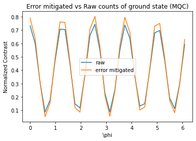
We can see how the error mitigated results yield a far greater fidelity than the raw data

zeros_m = [(1/shots)*result_exp_em.get_counts(a)[zerocode] if
          zerocode in result_exp_em.get_counts(a) else 0 for a in range(len(sweep)) ]

Plotter('mqc').sin_plotter(sweep,zeros,zeros_m)

Plotter('mqc').get_fourier_info(qn,sweep,zeros,zeros_m,p_dict)

Upper/Lower raw fidelity bounds =  0.859  +/-  0.009  ||  0.803  +/- 0.008
Upper/Lower error mitigated fidelity bounds =  0.893  +/-  0.009  ||  0.859  +/-  0.009
Raw fidelity =  0.843  +/-  0.008
Mitigated fidelity =  0.871  +/-  0.009

{'I0': (0.418212890625+0j),
 'In': (0.16118166625237523-0.0012795073482437993j),
 'I0_m': (0.4308643685037955+0j),
 'In_m': (0.18429327319353733-0.0014090290842254504j),
 'LB': 0.8029613807019665,
 'UB': 0.8587622724341675,
 'LB_m': 0.8586003949162327,
 'UB_m': 0.8934469245303837,
 'F': 0.8427021681078096,
 'F_m': 0.8705216752149427}

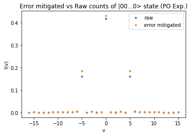
We now plot the DFT and compare the heights of the peaks to give bounds for the fidelity

Statistical bootstrapping has found that the error on these measurements is at most 1.5% (arXiv 1905.05720), so these result fall within error bounds, despite the fidelity being slightly higher than the upper bound, and show how error mitigation dramatically increases fidelity

Part 2: Parity Oscillation

We now retrieve a parallelized Parity Oscillation circuit for the n qubit device, and run experiments in the same fashion as we did in MQC.

shots = 1024
max_credits = 3
qn = 5
zerocode = '0'*qn
sweep = np.arange(0,np.pi*2,np.pi/16)

%%time
circ, [theta,thetaneg] , initial_layout = protocirc.get_ghz_po_para(qn)

circ_total = [circ.bind_parameters({theta:t, thetaneg:-t}) for t in sweep]

CPU times: user 2.02 s, sys: 38.5 ms, total: 2.06 s
Wall time: 2.06 s

job_exp = execute(circ_total, backend, shots=shots, max_credits=max_credits,
                  noise_model=noise_model, coupling_map=coupling_map, basis_gates=basis_gates)
job_monitor(job_exp)
result_exp = job_exp.result()

Job Status: job has successfully run

Now we construct the \(\otimes _{j}^{N} \sigma_z^{j}\) matrix for instruction, although this is already taken into account in the following method, entanglement.analysis.composite_pauli_z_expvalue():

composite_sigma_z = sigma_z = np.array([[1, 0],[0, -1]])
for a in range(1,qn):
    composite_sigma_z = np.kron(composite_sigma_z,sigma_z)

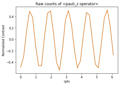
Now we want to make sure that our list of counts is correctly ordered so that it coincides with the states of the \(\otimes _{j}^{N} \sigma_z^{j}\), so that calculating \(\langle \otimes _{j}^{N} \sigma_z^{j} \rangle\) will be as simple as taking the dot product of this ordered list with the diagonal of \(\otimes _{j}^{N} \sigma_z^{j}\). The composite_pauli_z_expvalue function does just that; it takes a circuit and appropriately orders the state vector counts. We can plot this dot product as a function of \(\phi\) to observe parity oscillations.

from qiskit.ignis.verification.entanglement.analysis import composite_pauli_z_expvalue

y = [ (1/shots)*composite_pauli_z_expvalue(result_exp.get_counts(i),qn) for i in range(len(sweep))]

plt.plot(sweep,y)
Plotter('po').sin_plotter(sweep,y)

Now for standard error mitigation:

qr = QuantumRegister(qn)
qubit_list = range(qn)
meas_calibs, state_labels = complete_meas_cal(qubit_list=qubit_list, qr=qr, circlabel='mcal')

job_cal = execute(meas_calibs, backend=backend,
                  noise_model=noise_model, coupling_map=coupling_map, basis_gates=basis_gates)
job_monitor(job_cal)
meas_result = job_cal.result()

Job Status: job has successfully run

meas_fitter = CompleteMeasFitter(meas_result,state_labels,circlabel='mcal')
result_exp_em = meas_fitter.filter.apply(result_exp)

y_m = [ (1/shots)*composite_pauli_z_expvalue(result_exp_em.get_counts(i),qn) for i in range(len(sweep))]

Plotter('po').sin_plotter(sweep,y,y_m)

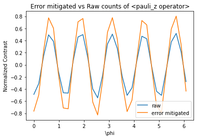
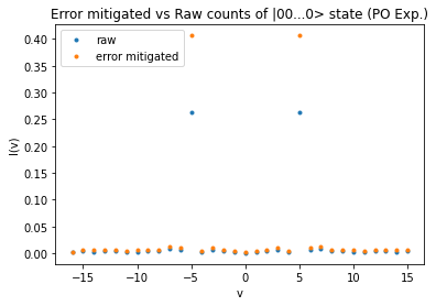
We can see how error mitigation dramatically improves our measurement (much more so in PO than in MQC). Let us quantify this using the same DFT method we used in MQC, and calculating the actual fidelities:

Plotter('po').get_fourier_info(qn,sweep,y,y_m,p_dict)

Raw fidelity =  0.628  +/-  0.006
Mitigated fidelity =  0.848  +/-  0.008

{'In': (-0.262421772178998-0.0006775920520316926j),
 'In_m': (-0.4065802411692412-0.001352956030108857j),
 'F': 0.6276570219734556,
 'F_m': 0.8478039700007223}

As we see, the raw fidelity is much lower than what is achieved with MQC, but the error mitigated result is about the same.

Part 3: Tomography

The first step in this experiment to just pass a simple GHZ state with no measurements. Also, the circuit cannot be transpiled; the transpiled argument in the getGHZChecker() method can be turned on and off as is shown

shots = 1024
max_credits = 3
qn = 5
zerocode = '0'*qn
q = QuantumRegister(qn, 'q')

circ_total, initial_layout = protocirc.get_ghz_layout(qn,transpiled=False)

We now pass a simulated backend from Aer to get theoretical statevector counts

job_exp = execute(circ_total, Aer.get_backend('statevector_simulator'), shots=shots, max_credits=max_credits)
job_monitor(job_exp)
result_exp = job_exp.result()
psi_exp = result_exp.get_statevector(circ_total)

Job Status: job has successfully run

This following code runs tomography experiments on the circuit we defined first, which is then compared to the theoretical statevector to generate a density matrix

qst = state_tomography_circuits(circ_total,q)
job = execute(qst, backend, shots=shots, initial_layout=initial_layout,noise_model=noise_model, coupling_map=coupling_map, basis_gates=basis_gates)
job_monitor(job)

Job Status: job has successfully run

tomo = StateTomographyFitter(job.result(), qst)

From here we can get the fidelity, although this method is not as fool proof as the one we will get to eventually:

F = quantum_info.state_fidelity(psi_exp,tomo.fit(), validate=False)

…And now for error mitigation…

qr = QuantumRegister(qn)
qubit_list = range(qn)
meas_calibs, state_labels = complete_meas_cal(qubit_list=qubit_list, qr=qr, circlabel='mcal')

job_c = execute(meas_calibs, backend=backend,
                  noise_model=noise_model, coupling_map=coupling_map, basis_gates=basis_gates)
job_monitor(job_c)
meas_result = job_c.result()

Job Status: job has successfully run

meas_fitter = CompleteMeasFitter(meas_result,state_labels,circlabel='mcal')
result_em = meas_fitter.filter.apply(job.result())

result_em = meas_fitter.filter.apply(job.result())
tomo_em = StateTomographyFitter(result_em, qst)

Now, using qiskit.visualization, we can plot the raw density matrix, real, and imaginary parts being on separate plots,…

visualization.plot_state_city(tomo.fit(),"city")

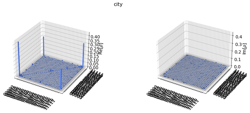
And also the error mitigated density matrix,…

visualization.plot_state_city(tomo_em.fit(),"city")

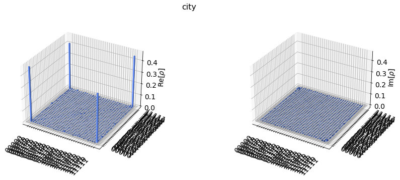
The actual density matrices can be obtained using the fit() method. Once we have the density matrix, we can compute the fidelity, which is nothing but half the sum of the four corners of the density matrix; the following method helps us:

from qiskit.ignis.verification.entanglement.analysis import rho_to_fidelity

rho, rho_em = tomo.fit() , tomo_em.fit()

F = rho_to_fidelity(rho)
F_em = rho_to_fidelity(rho_em)

print("Raw fidelity: ",F)
print("Error mitigated fidelity: ",F_em)

Raw fidelity:  0.6309007771150085
Error mitigated fidelity:  0.8718919315870092

As we see, the raw fidelity is much lower than what is achieved with either MQC or Parity Oscillations, but the error mitigated result is about the same.

A note on tomography

Do not perform quantum tomography with >5 qubits

Conclusion

In conclusion, we see that without error mitigation, MQC is the superior method for characterizing the GHZ state. However, with error mitigation, all methods can, at least for a small number of qubits, achieve a much greater fidelity, and all near the same value. To get more accurate results, aside from using a real device, it is worth increasing the number of shots four to eight-fold. It may be worth comparing how the parallelized circuits used in this notebook perform fidelity-wise versus linearized circuits.

External collaborators

Rohith Karur

import qiskit.tools.jupyter
%qiskit_version_table
%qiskit_copyright

/home/computertreker/git/qiskit/qiskit/.tox/docs/lib/python3.7/site-packages/qiskit/aqua/__init__.py:86: DeprecationWarning: The package qiskit.aqua is deprecated. It was moved/refactored to qiskit-terra For more information see <https://github.com/Qiskit/qiskit-aqua/blob/main/README.md#migration-guide>
  warn_package('aqua', 'qiskit-terra')

Version Information

Qiskit Software	Version
qiskit-terra	0.18.2
qiskit-aer	0.8.2
qiskit-ignis	0.6.0
qiskit-ibmq-provider	0.16.0
qiskit-aqua	0.9.5
qiskit	0.29.1
qiskit-nature	0.2.2
qiskit-finance	0.3.0
qiskit-optimization	0.2.3
qiskit-machine-learning	0.2.1
System information
Python	3.7.12 (default, Nov 22 2021, 14:57:10) [GCC 11.1.0]
OS	Linux
CPUs	32
Memory (Gb)	125.71650314331055
Tue Jan 04 11:16:28 2022 EST

This code is a part of Qiskit

© Copyright IBM 2017, 2022.

This code is licensed under the Apache License, Version 2.0. You may
obtain a copy of this license in the LICENSE.txt file in the root directory
of this source tree or at http://www.apache.org/licenses/LICENSE-2.0.

Any modifications or derivative works of this code must retain this
copyright notice, and modified files need to carry a notice indicating
that they have been altered from the originals.