Note

This page was generated from tutorials/circuits_advanced/06_building_pulse_schedules.ipynb.

Building Pulse Schedules

Pulse gates define a low-level, exact representation for a circuit gate. A single operation can be implemented with a pulse program, which is comprised of multiple low-level instructions. To learn more about pulse gates, refer back to the documentation here. This page details how to create pulse programs.

Note: For IBM devices, pulse programs are used as subroutines to describe gates. Previously, some devices accepted full programs in this format, but this is being sunset in December 2021. Other providers may still accept full programs in this format. Regardless of how the program is used, the syntax for building the program is the same. Read on to learn how!

Pulse programs, which are called Schedules, describe instruction sequences for the control electronics. We build Schedules using the Pulse Builder. It’s easy to initialize a schedule:

from qiskit import pulse

with pulse.build(name='my_example') as my_program:
    # Add instructions here
    pass

my_program

ScheduleBlock(, name="my_example", transform=AlignLeft())

You can see that there are no instructions yet. The next section of this page will explain each of the instructions you might add to a schedule, and the last section will describe various alignment contexts, which determine how instructions are placed in time relative to one another.

Schedule Instructions

• delay(duration, channel)

• play(pulse, channel)

• set_frequency(frequency, channel)

• shift_phase(phase, channel)

• acquire(duration, channel, mem_slot, reg_slot)

Each instruction type has its own set of operands. As you can see above, they each include at least one Channel to specify where the instruction will be applied.

Channels are labels for signal lines from the control hardware to the quantum chip.

• DriveChannels are typically used for driving single qubit rotations,

• ControlChannels are typically used for multi-qubit gates or additional drive lines for tunable qubits,

• MeasureChannels are specific to transmitting pulses which stimulate readout, and

• AcquireChannels are used to trigger digitizers which collect readout signals.

DriveChannels, ControlChannels, and MeasureChannels are all PulseChannels; this means that they support transmitting pulses, whereas the AcquireChannel is a receive channel only and cannot play waveforms.

For the following examples, we will create one DriveChannel instance for each Instruction that accepts a PulseChannel. Channels take one integer index argument. Except for ControlChannels, the index maps trivially to the qubit label.

from qiskit.pulse import DriveChannel

channel = DriveChannel(0)

The pulse Schedule is independent of the backend it runs on. However, we can build our program in a context that is aware of the target backend by supplying it to pulse.build. When possible you should supply a backend. By using the channel accessors pulse.<type>_channel(<idx>) we can make sure we are only using available device resources.

from qiskit.test.mock import FakeValencia

backend = FakeValencia()

with pulse.build(backend=backend, name='backend_aware') as backend_aware_program:
    channel = pulse.drive_channel(0)
    print(pulse.num_qubits())
    # Raises an error as backend only has 5 qubits
    #pulse.drive_channel(100)

5

delay

One of the simplest instructions we can build is delay. This is a blocking instruction that tells the control electronics to output no signal on the given channel for the duration specified. It is useful for controlling the timing of other instructions.

The duration here and elsewhere is in terms of the backend’s cycle time (1 / sample rate), dt. It must take an integer value.

To add a delay instruction, we pass a duration and a channel, where channel can be any kind of channel, including AcquireChannel. We use pulse.build to begin a Pulse Builder context. This automatically schedules our delay into the schedule delay_5dt.

with pulse.build(backend) as delay_5dt:
    pulse.delay(5, channel)

That’s all there is to it. Any instruction added after this delay on the same channel will execute five timesteps later than it would have without this delay.

play

The play instruction is responsible for executing pulses. It’s straightforward to add a play instruction:

with pulse.build() as sched:
    pulse.play(pulse, channel)

Let’s clarify what the pulse argument is and explore a few different ways to build one.

Pulses

A Pulse specifies an arbitrary pulse envelope. The modulation frequency and phase of the output waveform are controlled by the set_frequency and shift_phase instructions, which we will cover next.

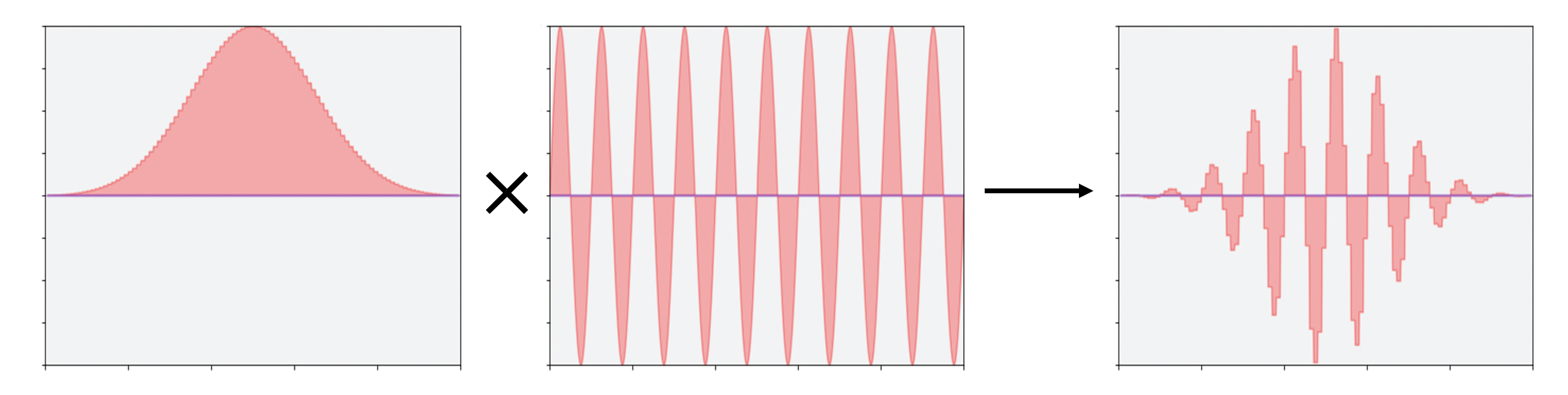
The image below may provide some intuition for why they are specified separately. Think of the pulses which describe their envelopes as input to an arbitrary waveform generator (AWG), a common lab instrument – this is depicted in the left image. Notice the limited sample rate discritizes the signal. The signal produced by the AWG may be mixed with a continuous sine wave generator. The frequency of its output is controlled by instructions to the sine wave generator; see the middle image. Finally, the signal sent to the qubit is demonstrated by the right side of the image below.

Note: The hardware may be implemented in other ways, but if we keep the instructions separate, we avoid losing explicit information, such as the value of the modulation frequency.

There are many methods available to us for building up pulses. Our library within Qiskit Pulse contains helpful methods for building Pulses. Let’s take for example a simple Gaussian pulse – a pulse with its envelope described by a sampled Gaussian function. We arbitrarily choose an amplitude of 1, standard deviation \(\sigma\) of 10, and 128 sample points.

Note: The amplitude norm is arbitrarily limited to 1.0. Each backend system may also impose further constraints – for instance, a minimum pulse size of 64. These additional constraints, if available, would be provided through the BackendConfiguration which is described here.

from qiskit.pulse import library

amp = 1
sigma = 10
num_samples = 128

Parametric pulses

Let’s build our Gaussian pulse using the Gaussian parametric pulse. A parametric pulse sends the name of the function and its parameters to the backend, rather than every individual sample. Using parametric pulses makes the jobs you send to the backend much smaller. IBM Quantum backends limit the maximum job size that they accept, so parametric pulses may allow you to run larger programs.

Other parametric pulses in the library include GaussianSquare, Drag, and Constant.

Note: The backend is responsible for deciding exactly how to sample the parametric pulses. It is possible to draw parametric pulses, but the samples displayed are not guaranteed to be the same as those executed on the backend.

gaus = pulse.library.Gaussian(num_samples, amp, sigma,
                              name="Parametric Gaus")
gaus.draw()

Pulse waveforms described by samples

A Waveform is a pulse signal specified as an array of time-ordered complex amplitudes, or samples. Each sample is played for one cycle, a timestep dt, determined by the backend. If we want to know the real-time dynamics of our program, we need to know the value of dt. The (zero-indexed) \(i^{th}\) sample will play from time i*dt up to (i + 1)*dt, modulated by the qubit frequency.

import numpy as np

times = np.arange(num_samples)
gaussian_samples = np.exp(-1/2 *((times - num_samples / 2) ** 2 / sigma**2))

gaus = library.Waveform(gaussian_samples, name="WF Gaus")
gaus.draw()

Pulse library functions

Our own pulse library has sampling methods to build a Waveform from common functions.

gaus = library.gaussian(duration=num_samples, amp=amp, sigma=sigma, name="Lib Gaus")
gaus.draw()

Regardless of which method you use to specify your pulse, play is added to your schedule the same way:

with pulse.build() as schedule:
    pulse.play(gaus, channel)
schedule.draw()

You may also supply a complex list or array directly to play

with pulse.build() as schedule:
    pulse.play([0.001*i for i in range(160)], channel)
schedule.draw()

The play instruction gets its duration from its Pulse: the duration of a parametrized pulse is an explicit argument, and the duration of a Waveform is the number of input samples.

set_frequency

As explained previously, the output pulse waveform envelope is also modulated by a frequency and phase. Each channel has a default frequency listed in the backend.defaults().

The frequency of a channel can be updated at any time within a Schedule by the set_frequency instruction. It takes a float frequency and a PulseChannel channel as input. All pulses on a channel following a set_frequency instruction will be modulated by the given frequency until another set_frequency instruction is encountered or until the program ends.

The instruction has an implicit duration of 0.

Note: The frequencies that can be requested are limited by the total bandwidth and the instantaneous bandwidth of each hardware channel. In the future, these will be reported by the backend.

with pulse.build(backend) as schedule:
    pulse.set_frequency(4.5e9, channel)

shift_phase

The shift_phase instruction will increase the phase of the frequency modulation by phase. Like set_frequency, this phase shift will affect all following instructions on the same channel until the program ends. To undo the affect of a shift_phase, the negative phase can be passed to a new instruction.

Like set_frequency, the instruction has an implicit duration of 0.

with pulse.build(backend) as schedule:
    pulse.shift_phase(np.pi, channel)

acquire

The acquire instruction triggers data acquisition for readout. It takes a duration, an AcquireChannel which maps to the qubit being measured, and a MemorySlot or a RegisterSlot. The MemorySlot is classical memory where the readout result will be stored. The RegisterSlot maps to a register in the control electronics which stores the readout result for fast feedback.

The acquire instructions can also take custom Discriminators and Kernels as keyword arguments.

from qiskit.pulse import Acquire, AcquireChannel, MemorySlot

with pulse.build(backend) as schedule:
    pulse.acquire(1200, pulse.acquire_channel(0), MemorySlot(0))

Now that we know how to add Schedule instructions, let’s learn how to control exactly when they’re played.

Pulse Builder

Here, we will go over the most important Pulse Builder features for learning how to build schedules. This is not exhaustive; for more details about what you can do using the Pulse Builder, check out the Pulse API reference.

Alignment contexts

The builder has alignment contexts which influence how a schedule is built. Contexts can also be nested. Try them out, and use .draw() to see how the pulses are aligned.

Regardless of the alignment context, the duration of the resulting schedule is as short as it can be while including every instruction and following the alignment rules. This still allows some degrees of freedom for scheduling instructions off the “longest path”. The examples below illuminate this.

align_left

The builder has alignment contexts that influence how a schedule is built. The default is align_left.

with pulse.build(backend, name='Left align example') as program:
    with pulse.align_left():
        gaussian_pulse = library.gaussian(100, 0.5, 20)
        pulse.play(gaussian_pulse, pulse.drive_channel(0))
        pulse.play(gaussian_pulse, pulse.drive_channel(1))
        pulse.play(gaussian_pulse, pulse.drive_channel(1))

program.draw()

Notice how there is no scheduling freedom for the pulses on D1. The second waveform begins immediately after the first. The pulse on D0 can start at any time between t=0 and t=100 without changing the duration of the overall schedule. The align_left context sets the start time of this pulse to t=0. You can think of this like left-justification of a text document.

align_right

Unsurprisingly, align_right does the opposite of align_left. It will choose t=100 in the above example to begin the gaussian pulse on D0. Left and right are also sometimes called “as soon as possible” and “as late as possible” scheduling, respectively.

with pulse.build(backend, name='Right align example') as program:
    with pulse.align_right():
        gaussian_pulse = library.gaussian(100, 0.5, 20)
        pulse.play(gaussian_pulse, pulse.drive_channel(0))
        pulse.play(gaussian_pulse, pulse.drive_channel(1))
        pulse.play(gaussian_pulse, pulse.drive_channel(1))

program.draw()

align_equispaced(duration)

If the duration of a particular block is known, you can also use align_equispaced to insert equal duration delays between each instruction.

with pulse.build(backend, name='example') as program:
    gaussian_pulse = library.gaussian(100, 0.5, 20)
    with pulse.align_equispaced(2*gaussian_pulse.duration):
        pulse.play(gaussian_pulse, pulse.drive_channel(0))
    pulse.play(gaussian_pulse, pulse.drive_channel(1))
    pulse.play(gaussian_pulse, pulse.drive_channel(1))

program.draw()

align_sequential

This alignment context does not schedule instructions in parallel. Each instruction will begin at the end of the previously added instruction.

with pulse.build(backend, name='example') as program:
    with pulse.align_sequential():
        gaussian_pulse = library.gaussian(100, 0.5, 20)
        pulse.play(gaussian_pulse, pulse.drive_channel(0))
        pulse.play(gaussian_pulse, pulse.drive_channel(1))
        pulse.play(gaussian_pulse, pulse.drive_channel(1))

program.draw()

Phase and frequency offsets

We can use the builder to help us temporarily offset the frequency or phase of our pulses on a channel.

with pulse.build(backend, name='Offset example') as program:
    with pulse.phase_offset(3.14, pulse.drive_channel(0)):
        pulse.play(gaussian_pulse, pulse.drive_channel(0))
        with pulse.frequency_offset(10e6, pulse.drive_channel(0)):
            pulse.play(gaussian_pulse, pulse.drive_channel(0))

program.draw()

We encourage you to visit the Pulse API reference to learn more.

import qiskit.tools.jupyter
%qiskit_version_table
%qiskit_copyright

/home/computertreker/git/qiskit/qiskit/.tox/docs/lib/python3.7/site-packages/qiskit/aqua/__init__.py:86: DeprecationWarning: The package qiskit.aqua is deprecated. It was moved/refactored to qiskit-terra For more information see <https://github.com/Qiskit/qiskit-aqua/blob/main/README.md#migration-guide>
  warn_package('aqua', 'qiskit-terra')

Version Information

Qiskit Software	Version
qiskit-terra	0.18.2
qiskit-aer	0.8.2
qiskit-ignis	0.6.0
qiskit-ibmq-provider	0.16.0
qiskit-aqua	0.9.5
qiskit	0.29.1
qiskit-nature	0.2.2
qiskit-finance	0.3.0
qiskit-optimization	0.2.3
qiskit-machine-learning	0.2.1
System information
Python	3.7.12 (default, Nov 22 2021, 14:57:10) [GCC 11.1.0]
OS	Linux
CPUs	32
Memory (Gb)	125.71650314331055
Tue Jan 04 11:07:28 2022 EST

This code is a part of Qiskit

© Copyright IBM 2017, 2022.

This code is licensed under the Apache License, Version 2.0. You may
obtain a copy of this license in the LICENSE.txt file in the root directory
of this source tree or at http://www.apache.org/licenses/LICENSE-2.0.

Any modifications or derivative works of this code must retain this
copyright notice, and modified files need to carry a notice indicating
that they have been altered from the originals.