Note

This page was generated from tutorials/circuits/01_circuit_basics.ipynb.

Circuit Basics¶

Here, we provide an overview of working with Qiskit. Qiskit provides the basic building blocks necessary to program quantum computers. The fundamental unit of Qiskit is the quantum circuit. A basic workflow using Qiskit consists of two stages: Build and Run. Build allows you to make different quantum circuits that represent the problem you are solving, and Run that allows you to run them on different backends. After the jobs have been run, the data is collected and postprocessed depending on the desired output.

[1]:

import numpy as np
from qiskit import QuantumCircuit

Building the circuit¶

The basic element needed for your first program is the QuantumCircuit. We begin by creating a QuantumCircuit comprised of three qubits.

[2]:

# Create a Quantum Circuit acting on a quantum register of three qubits
circ = QuantumCircuit(3)

After you create the circuit with its registers, you can add gates (“operations”) to manipulate the registers. As you proceed through the tutorials you will find more gates and circuits; below is an example of a quantum circuit that makes a three-qubit GHZ state

\[|\psi\rangle = \left(|000\rangle+|111\rangle\right)/\sqrt{2}.\]

To create such a state, we start with a three-qubit quantum register. By default, each qubit in the register is initialized to $|0\rangle$. To make the GHZ state, we apply the following gates: - A Hadamard gate $H$ on qubit 0, which puts it into the superposition state $\left(|0\rangle+|1\rangle\right)/\sqrt{2}$. - A controlled-Not operation ($C_{X}$) between qubit 0 and qubit 1. - A controlled-Not operation between qubit 0 and qubit 2.

On an ideal quantum computer, the state produced by running this circuit would be the GHZ state above.

In Qiskit, operations can be added to the circuit one by one, as shown below.

[3]:

# Add a H gate on qubit 0, putting this qubit in superposition.
circ.h(0)
# Add a CX (CNOT) gate on control qubit 0 and target qubit 1, putting
# the qubits in a Bell state.
circ.cx(0, 1)
# Add a CX (CNOT) gate on control qubit 0 and target qubit 2, putting
# the qubits in a GHZ state.
circ.cx(0, 2)

[3]:

<qiskit.circuit.instructionset.InstructionSet at 0x7fb48e05b110>

Visualize Circuit¶

You can visualize your circuit using Qiskit QuantumCircuit.draw(), which plots the circuit in the form found in many textbooks.

[4]:

circ.draw('mpl')

[4]:

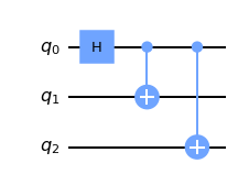
../../_images/tutorials_circuits_01_circuit_basics_7_0.png

In this circuit, the qubits are put in order, with qubit zero at the top and qubit two at the bottom. The circuit is read left to right (meaning that gates that are applied earlier in the circuit show up further to the left).

When representing the state of a multi-qubit system, the tensor order used in Qiskit is different than that used in most physics textbooks. Suppose there are $n$ qubits, and qubit $j$ is labeled as $Q_{j}$. Qiskit uses an ordering in which the $n^{\mathrm{th}}$ qubit is on the left side of the tensor product, so that the basis vectors are labeled as $Q_{n-1}\otimes \cdots \otimes Q_1\otimes Q_0$.

For example, if qubit zero is in state 0, qubit 1 is in state 0, and qubit 2 is in state 1, Qiskit would represent this state as $|100\rangle$, whereas many physics textbooks would represent it as $|001\rangle$.

This difference in labeling affects the way multi-qubit operations are represented as matrices. For example, Qiskit represents a controlled-X ($C_{X}$) operation with qubit 0 being the control and qubit 1 being the target as

\[\begin{split}C_X = \begin{pmatrix} 1 & 0 & 0 & 0 \\ 0 & 0 & 0 & 1 \\ 0 & 0 & 1 & 0 \\ 0 & 1 & 0 & 0 \\\end{pmatrix}.\end{split}\]

Simulating circuits¶

To simulate a circuit we use the quant_info module in Qiskit. This simulator returns the quantum state, which is a complex vector of dimensions $2^n$, where $n$ is the number of qubits (so be careful using this as it will quickly get too large to run on your machine).

There are two stages to the simulator. The first is to set the input state and the second to evolve the state by the quantum circuit.

[5]:

from qiskit.quantum_info import Statevector

# Set the intial state of the simulator to the ground state using from_int
state = Statevector.from_int(0, 2**3)

# Evolve the state by the quantum circuit
state = state.evolve(circ)

#draw using latex
state.draw('latex')

[5]:

$$ \begin{bmatrix} \tfrac{1}{\sqrt{2}} & 0 & 0 & 0 & 0 & 0 & 0 & \tfrac{1}{\sqrt{2}} \\ \end{bmatrix} $$

[6]:

from qiskit.visualization import array_to_latex

#Alternative way of representing in latex
array_to_latex(state)

[6]:

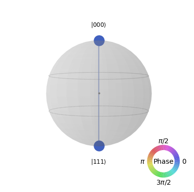
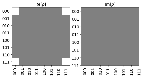
$$ \begin{bmatrix} \tfrac{1}{\sqrt{2}} & 0 & 0 & 0 & 0 & 0 & 0 & \tfrac{1}{\sqrt{2}} \\ \end{bmatrix} $$

Qiskit also provides a visualization toolbox to allow you to view the state.

Below, we use the visualization function to plot the qsphere and a hinton representing the real and imaginary components of the state density matrix $\rho$.

[7]:

state.draw('qsphere')

[7]:

../../_images/tutorials_circuits_01_circuit_basics_14_0.png

[8]:

state.draw('hinton')

[8]:

../../_images/tutorials_circuits_01_circuit_basics_15_0.png

Unitary representation of a circuit¶

Qiskit’s quant_info module also has an operator method which can be used to make a unitary operator for the circuit. This calculates the $2^n \times 2^n$ matrix representing the quantum circuit.

[9]:

from qiskit.quantum_info import Operator

U = Operator(circ)

# Show the results
U.data

[9]:

array([[ 0.70710678+0.j,  0.70710678+0.j,  0.        +0.j,
         0.        +0.j,  0.        +0.j,  0.        +0.j,
         0.        +0.j,  0.        +0.j],
       [ 0.        +0.j,  0.        +0.j,  0.        +0.j,
         0.        +0.j,  0.        +0.j,  0.        +0.j,
         0.70710678+0.j, -0.70710678+0.j],
       [ 0.        +0.j,  0.        +0.j,  0.70710678+0.j,
         0.70710678+0.j,  0.        +0.j,  0.        +0.j,
         0.        +0.j,  0.        +0.j],
       [ 0.        +0.j,  0.        +0.j,  0.        +0.j,
         0.        +0.j,  0.70710678+0.j, -0.70710678+0.j,
         0.        +0.j,  0.        +0.j],
       [ 0.        +0.j,  0.        +0.j,  0.        +0.j,
         0.        +0.j,  0.70710678+0.j,  0.70710678+0.j,
         0.        +0.j,  0.        +0.j],
       [ 0.        +0.j,  0.        +0.j,  0.70710678+0.j,
        -0.70710678+0.j,  0.        +0.j,  0.        +0.j,
         0.        +0.j,  0.        +0.j],
       [ 0.        +0.j,  0.        +0.j,  0.        +0.j,
         0.        +0.j,  0.        +0.j,  0.        +0.j,
         0.70710678+0.j,  0.70710678+0.j],
       [ 0.70710678+0.j, -0.70710678+0.j,  0.        +0.j,
         0.        +0.j,  0.        +0.j,  0.        +0.j,
         0.        +0.j,  0.        +0.j]])

OpenQASM backend¶

The simulators above are useful because they provide information about the state output by the ideal circuit and the matrix representation of the circuit. However, a real experiment terminates by measuring each qubit (usually in the computational $|0\rangle, |1\rangle$ basis). Without measurement, we cannot gain information about the state. Measurements cause the quantum system to collapse into classical bits.

For example, suppose we make independent measurements on each qubit of the three-qubit GHZ state

\[|\psi\rangle = (|000\rangle +|111\rangle)/\sqrt{2},\]

and let $xyz$ denote the bitstring that results. Recall that, under the qubit labeling used by Qiskit, $x$ would correspond to the outcome on qubit 2, $y$ to the outcome on qubit 1, and $z$ to the outcome on qubit 0.

Note: This representation of the bitstring puts the most significant bit (MSB) on the left, and the least significant bit (LSB) on the right. This is the standard ordering of binary bitstrings. We order the qubits in the same way (qubit representing the MSB has index 0), which is why Qiskit uses a non-standard tensor product order.

Recall the probability of obtaining outcome $xyz$ is given by

\[\mathrm{Pr}(xyz) = |\langle xyz | \psi \rangle |^{2}\]

and as such for the GHZ state probability of obtaining 000 or 111 are both 1/2.

To simulate a circuit that includes measurement, we need to add measurements to the original circuit above, and use a different Aer backend.

[10]:

# Create a Quantum Circuit
meas = QuantumCircuit(3, 3)
meas.barrier(range(3))
# map the quantum measurement to the classical bits
meas.measure(range(3), range(3))

# The Qiskit circuit object supports composition.
# Here the meas has to be first and front=True (putting it before)
# as compose must put a smaller circuit into a larger one.
qc = meas.compose(circ, range(3), front=True)

#drawing the circuit
qc.draw('mpl')

[10]:

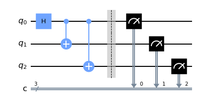
../../_images/tutorials_circuits_01_circuit_basics_21_0.png

This circuit adds a classical register, and three measurements that are used to map the outcome of qubits to the classical bits.

To simulate this circuit, we use the qasm_simulator in Qiskit Aer. Each run of this circuit will yield either the bitstring 000 or 111. To build up statistics about the distribution of the bitstrings (to, e.g., estimate $\mathrm{Pr}(000)$), we need to repeat the circuit many times. The number of times the circuit is repeated can be specified in the execute function, via the shots keyword.

[11]:

# Adding the transpiler to reduce the circuit to QASM instructions
# supported by the backend
from qiskit import transpile

# Use Aer's qasm_simulator
from qiskit.providers.aer import QasmSimulator

backend = QasmSimulator()

# First we have to transpile the quantum circuit
# to the low-level QASM instructions used by the
# backend
qc_compiled = transpile(qc, backend)

# Execute the circuit on the qasm simulator.
# We've set the number of repeats of the circuit
# to be 1024, which is the default.
job_sim = backend.run(qc_compiled, shots=1024)

# Grab the results from the job.
result_sim = job_sim.result()

Once you have a result object, you can access the counts via the function get_counts(circuit). This gives you the aggregated binary outcomes of the circuit you submitted.

[12]:

counts = result_sim.get_counts(qc_compiled)
print(counts)

{'111': 548, '000': 476}

Approximately 50 percent of the time, the output bitstring is 000. Qiskit also provides a function plot_histogram, which allows you to view the outcomes.

[13]:

from qiskit.visualization import plot_histogram
plot_histogram(counts)

[13]:

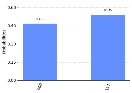
../../_images/tutorials_circuits_01_circuit_basics_27_0.png

The estimated outcome probabilities $\mathrm{Pr}(000)$ and $\mathrm{Pr}(111)$ are computed by taking the aggregate counts and dividing by the number of shots (times the circuit was repeated). Try changing the shots keyword in the execute function and see how the estimated probabilities change.

[14]:

import qiskit.tools.jupyter
%qiskit_version_table
%qiskit_copyright

/home/computertreker/git/qiskit/qiskit/.tox/docs/lib/python3.7/site-packages/qiskit/aqua/__init__.py:86: DeprecationWarning: The package qiskit.aqua is deprecated. It was moved/refactored to qiskit-terra For more information see <https://github.com/Qiskit/qiskit-aqua/blob/main/README.md#migration-guide>
  warn_package('aqua', 'qiskit-terra')

Version Information

Qiskit Software	Version
`qiskit-terra`	0.18.2
`qiskit-aer`	0.8.2
`qiskit-ignis`	0.6.0
`qiskit-ibmq-provider`	0.16.0
`qiskit-aqua`	0.9.5
`qiskit`	0.29.1
`qiskit-nature`	0.2.2
`qiskit-finance`	0.3.0
`qiskit-optimization`	0.2.3
`qiskit-machine-learning`	0.2.1
System information
Python	3.7.12 (default, Nov 22 2021, 14:57:10) [GCC 11.1.0]
OS	Linux
CPUs	32
Memory (Gb)	125.71650314331055
Tue Jan 04 11:05:49 2022 EST

This code is a part of Qiskit

This code is licensed under the Apache License, Version 2.0. You may
obtain a copy of this license in the LICENSE.txt file in the root directory
of this source tree or at http://www.apache.org/licenses/LICENSE-2.0.

Any modifications or derivative works of this code must retain this
copyright notice, and modified files need to carry a notice indicating
that they have been altered from the originals.